Introduction
In Part I, the magnetization admittance [1] was employed to calculate the fractional power lost to an FT140-43 ferrite core by a 10-turn winding at 21 MHz [2]. Part II will show how to calculate the amount of power the same ferrite core can dissipate into free air before reaching its Curie temperature. Modulation methods and duty factors will be figured into these calculations. Whether it is an inductor, transformer, or balun, the analysis is similar.
Although the maximum permissible ferrite temperature will not change as a function of the transmitting mode used, the maximum permissible amount of input transmitter power will. This subject will be explored in the context of ferrite transformers, including one sold by the ARRL for use in an end-fed half-wave antenna kit.
Recap
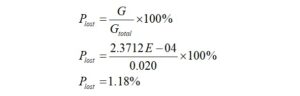
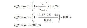
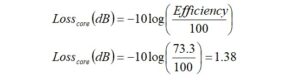
By way of review, it was shown in Part I that the percentage power lost to the ferrite core described in the introduction is given by,
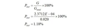
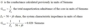
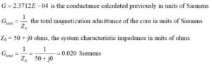
where:
The amount of power lost to the core is 1.18%.
While this is useful to know, we would also like to be able to calculate the amount of power that may be dissipated by the ferrite core to free air before the Curie temperature is reached. The Curie temperature is the temperature at which there are drastic changes in the material’s ferrimagnetic (Ferri, not Ferro) properties. When ferrite is used in the construction of antenna components, the Curie temperature will dictate what our transmitter operating power can be for specific modes and duty factors of operation.
Ferrite Core Efficiency
From the core loss, we may now calculate the efficiency from the expression,
This sounds like good efficiency, but it doesn’t take many Watts in a confined space to heat ferrite above its Curie temperature as will be shown.
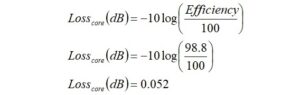
The core loss in dB is calculated from the expression,
Maximum Long-Term Average Power Dissipation
Case I
Next, we find the Curie temperature for #43 ferrite material from the datasheet [3],

We now consider the ambient operating temperature. For outdoor use in the summer, the ambient temperature inside an enclosure can easily rise to 50⁰C, and this may well be on the low side. It can easily be that hot in an attic during the summer.
If we take the Curie temperature and the ambient temperature into account, the allowable ferrite temperature rise is,

Next, we need to find a value for the convective heat transfer coefficient (HTC) for the ferrite into free air. The value offered by Owen Duffy [4] is,

This number appears in another paper [5] published by the U.S. Army Research Laboratory for ferrite subject to natural convection of 0.5 m/s, although 14 Watts/m2-K appears to be an upper limit.
Surface Area of a Toroid Core
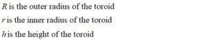
Next, we need to calculate the surface area of the ferrite toroid of a rectangular cross-section using the formula,

derived from the geometry of a hollow cylinder,
where:
Expanding the difference of squares and collecting terms obtains the simplified expression,

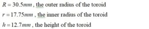
For an FT140-43 ferrite core, the dimensions are [6],
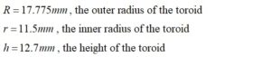
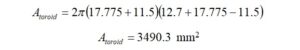
Recalling that 1 mm2 = 1E-6 m2

This area does not correct for any bevels or radii on the edges of the ferrite core.
The maximum long-term average power dissipation in Watts is given by,
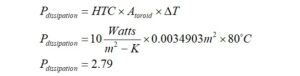
The maximum long-term average power dissipation is 2.79 Watts. This may come as a surprise, but that is all that it takes to cook this ferrite core if it is housed in a sealed box. At this point, it may be appropriate to advise that ferrite should be enclosed when subjected to even moderate amounts of power. Ferrite has been known to explode into shards. If more ventilation is required, enclosure manufacturers like Bud Industries make baffled vents for their enclosures. Some ferrite transformer manufacturers have recognized that vents should be added to their product lines.
Next, we need to calculate the maximum continuous average RF power in Watts that can be applied, which will result in a power dissipation of 2.79 Watts. This is given by the expression,

where:
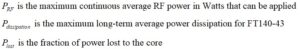

The maximum continuous average RF power that can be applied is 236.4 Watts.
Apparently, 10-turns on an FT140-43 core at 21 MHz is very efficient. That is due to the number of windings on the core, which tends to reduce flux leakage.
Case II
Next, we reduce the number of turns on the ferrite core to 2-turns, as is very often the case for transformer primary windings used to match end-fed half-wave antennas. Ultimately, we will need to calculate the value of conductance, G, for the new winding configuration at 21 MHz so that we may repeat the calculations.
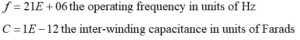
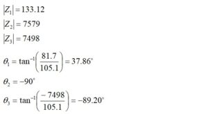
We start by calculating the impedance for the new configuration [7],

where:
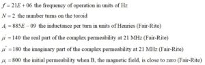
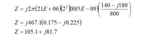
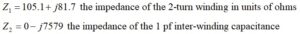
The impedance for a 2-turn transformer primary winding is 105.1+j81.7 ohms. We would like to place a 1 pf inter-winding capacitance in parallel with the primary impedance.
The capacitive reactance is calculated from,

where:

The capacitive reactance that will be in parallel with the impedance is 7579 ohms.
We calculate the parallel combination of two impedances using the formula

where:
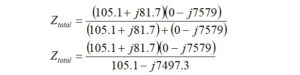
We could rationalize the denominator and simplify or convert it to polar form.
Let’s convert the impedances to polar form to arrive at the parallel combination. We define a new impedance for the denominator, Z3.
The capacitor has a phase angle θ2 = -90⁰ because the voltage lags the current.
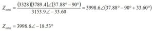
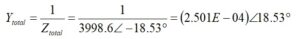
Now, we construct Ztotal in polar form,
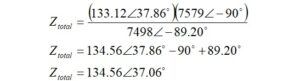
This is easily converted to admittance,

Note that the sign of the angle changes when it is moved to the numerator.
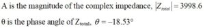
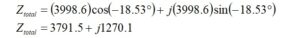
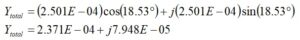
Converting back to rectangular form with the help of the Euler identity provides what is needed,
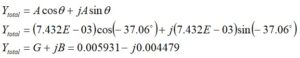
where:
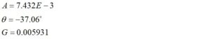
Once again, we calculate the power lost to the core,

Reducing the number of turns on the core has resulted in an enormous core loss.
The efficiency may be calculated,

The core loss in dB is,

The core loss is 1.53 dB.
The maximum long-term average power dissipation for the core does not change. It remains 2.79 Watts.
Now, we calculate the maximum continuous average RF power in Watts that can be applied which will result in long-term average power dissipation of 2.79 Watts.

The maximum continuous average RF power may not exceed 9.39 Watts.
Apparently, 2-turns on an FT140-43 core at 21 MHz is not very efficient. If we were to consider CW operation at a duty factor of 44%, we might be able to apply,

QRP operation on CW at 21 MHz should not be a problem.
For SSB that operates at an average power of about 10% PEP/Pavg, 93.9 Watts might be possible without overheating. This is a conservative number that includes speech compression. For uncompressed speech operating at 3% PEP/Pavg, 313 Watts might be possible.
Case III
Let’s analyze the case of the ARRL End-Fed Half-Wave Antenna Kit. The specifications state that this antenna is rated at 250 Watts PEP. The core used in the kit is an FT240-43. The turn ratio is 2:14 (1:7) for an impedance transformation of 1:49. The transformer is intended to match a 50-ohm source to a 2450 ohm load. The voltage requirement for the compensation capacitor in the kit will also be included in this analysis. Let’s assume operation at the very bottom of the 40m band, 7.0 MHz.
Surface Area of the Core

For an FT240-43 ferrite core, the dimensions are,
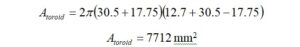
Recalling that 1 mm2 = 1E-6 m2

This area does not correct for any bevels or radii on the edges of the ferrite core.
Maximum Long-Term Average Power Dissipation
The maximum long-term average power dissipation in Watts is given by,
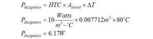
The larger FT240 core is capable of higher power dissipation before reaching the Curie temperature.
Primary Winding Impedance and Admittance
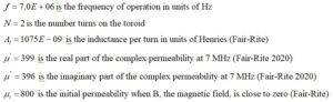
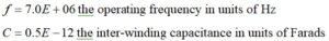
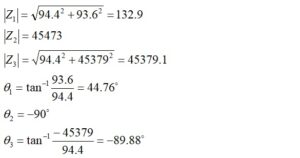
In order to calculate the efficiency of the FT240-43 core with 2 primary turns, the admittance will be required at 7 MHz. As before, we first calculate the impedance from the expression,

where:
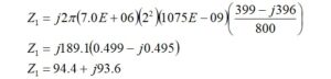
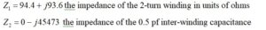
The impedance for a 2-turn transformer primary winding is 94.4+j93.6 ohms. We would like to place a 0.5 pf inter-winding capacitance in parallel with the primary impedance.
The capacitive reactance is calculated from

where:

The capacitive reactance that will be in parallel with the impedance is 45473 ohms. Thus, the impedance of the inter-winding capacitance is,

We calculate the parallel combination of two impedances using the formula,

where:
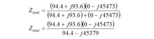
Again, we could rationalize the denominator by multiplying the top and bottom by the complex conjugate of the denominator or convert the top and bottom to polar form. Let’s convert to polar form and solve. We can assign impedance, Z3, to the denominator that has already been simplified.
Thus,
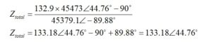
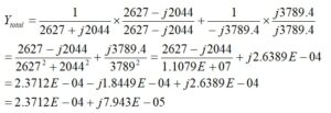
Please note that when the angle is moved from the denominator to the numerator, there is a sign change. We need the total admittance, and that is easy to calculate from,

Next, we convert the total admittance to rectangular form to recover the value of the conductance, G.
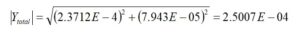
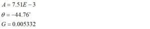
Converting back to rectangular form provides what is needed,
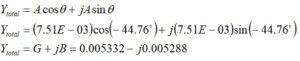
where:
Power Lost to the Core
Once again, we calculate the power lost to the core from,

The magnetization admittance loss is substantial at 7 MHz.
Core Efficiency
The efficiency may be calculated from,

Core Loss
The core loss in dB is,
The core loss is 1.38 dB.
Maximum Continuous Average RF Power
The maximum long-term average power dissipation for the core does not change. It remains 6.17 Watts.
Now, we calculate the maximum continuous average RF power in Watts that can be applied, which will result in a power dissipation of 6.17 Watts.

The maximum continuous average RF power may not exceed 23.1 Watts.
CW Operation
Apparently, 2-turns on an FT240-43 core at 7 MHz is not very efficient. If we were to consider CW operation at a duty factor of 44%, we might be able to apply,

QRP operation on CW at 7 MHz should not be a problem, but 100W CW operation would be a problem for a long tune-up and long-winded QSOs.
Uncompressed SSB operates at a 3% PEP/Pavg ratio [8], and that mode should be no problem at all for up to 769 Watts. Even in compressed audio operation at a 10% PEP/Pavg ratio [9], 231 Watts should not be an issue.
If we revisit everything in terms of Intermittent Commercial and Amateur Service (ICAS), everything changes. We find that the maximum continuous RF power becomes 46.2 Watts. CW operation becomes possible for up to 105 Watts. Uncompressed SSB operation is possible for up to 1538 Watts, and compressed SSB is possible for up to 462 Watts.
SSB looks like a success, while CW looks a bit marginal for all but short-duty QSOs during summer temperatures. At least for CW, operating habits contribute to success or failure.
Compensation Capacitor Voltage Rating
Next, let’s look at the capacitor used in the kit.
The ARRL kit is supplied with a compensation capacitor to be added to the transformer input. The instructions state that this capacitor may be omitted unless operation is required on the higher bands. It would be useful to know what its voltage rating should be under conditions of elevated VSWR [10]. The parts list tells us that the value of the capacitor is 100 pf and the voltage rating is 2 kV. This information is in the parts list. We are not told what the dielectric characteristics of the capacitor are.
If we assume operation in a system where the antenna mismatch is as bad as 6:1, we can calculate the maximum peak voltage on the transmission line that connects to the transformer input. The capacitor shunts the input. The calculations are performed for a 100 Watt transmitter.
Previously [11], it was demonstrated that the maximum peak voltage on a transmission line may be calculated from,

where:

VSWR is the voltage standing wave ratio on the transmission line
P0 is the power incident on the transformer, 100 Watts
Z0 is the characteristic impedance of the line, 50 ohms
If we assume a 6:1 VSWR, we can calculate the maximum peak voltage as,

If a 500 V capacitor were used, there would be more than 100% margin. The 2kV capacitor that is furnished with the kit far exceeds what is required.
Compensation Capacitor Dielectric Dissipation
It would also be useful to know how much dissipation there is in the capacitor. Poor quality ceramic capacitors possessing low Q can easily overheat.
Calculation of Q for a Capacitor
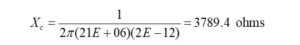
First, the magnitude of capacitive reactance at the desired operating frequency is calculated.

where:
For example, the value of Xc is calculated at 7 MHz for a 100 pf compensating capacitor. The capacitive reactance at 7 MHz for a 100 pf capacitor is,

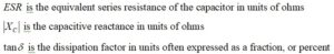
Next, the equivalent series resistance (ESR) of a capacitor may be calculated from the capacitive reactance and the dissipation factor,

where:
A typical Class III ceramic capacitor of 100 pf has a dissipation factor of 0.05 (5%) at 1 MHz, while a typical silvered mica capacitor has a dissipation factor of 0.00075 (0.075%) at 1 MHz. The dissipation factor does not change rapidly with frequency.
The ESR and Q for the Class III capacitor is calculated at 7 MHz,

where:
Q is the capacitor quality factor, dimensionless
Similarly, if the ESR and Q are calculated for a silvered mica capacitor at 7 MHz,

The lowest dissipation factor occurs for the silvered mica capacitor at 7 MHz as compared to the Class III ceramic capacitor.
Calculation of Dielectric Power Dissipation
In order to calculate the power dissipation for each type of capacitor, the equivalent shunt loss resistance is required,

For the ceramic capacitor, we obtain,

We repeat for the silvered mica capacitor,

The RMS voltage for 100 Watts into 50 ohms is given by,

The dissipations are for the ceramic capacitor,

and for the silvered mica capacitor,

It appears that a Class III capacitor is apt to cook if used as the compensation capacitor, while silvered mica parts might be a better choice. Better quality Class I ceramic and silvered mica capacitors with low dissipation factors are readily available.