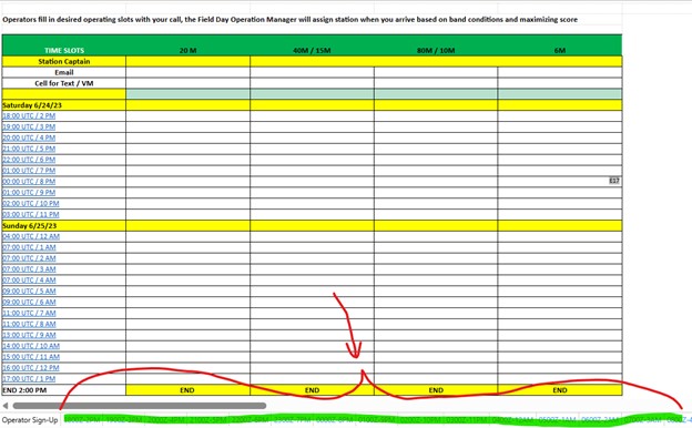
I’ve been off the air since moving back to NH in 2020. Since the landscaping has not been completed on the property, it has been impossible to install the radials for a 6-BTV vertical. Radials don’t fare well under the treads of a Bobcat.
A collection of single-band, matched, end-fed half-wave (EFHW) antennas was constructed while I was living in FL. All of these antennas underwent testing on an antenna range consisting of three 10m tall masts spaced 70 ft apart. These antennas were matched with L-networks. The test results were reported in a separate article[1].
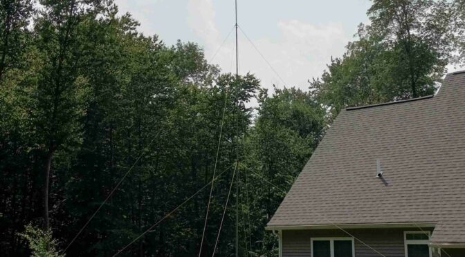
Seeing that July 4th weekend was approaching, I was eager to get on the air for a few days before the landscaper arrived. I decided on a 20m EFHW vertical that makes use of some of the guy ropes that were prepared for FL antenna testing. Figure 1 shows the installation of the 12.5m high telescoping fiberglass mast. The mast is anchored with a tilt-over base mounting plate described in a separate article[2]. Guying is provided at two levels. The guying radius is 25 ft. Guy anchoring is accomplished with polycarbonate Orange Screws[3]. While these anchors work well in FL sand, they do not work quite as well in rocky New England soil. I managed to snap one of them off in the process of screwing it into the ground.
My favorite knot for adjusting the guy rope tension is the taut-line hitch. I used the taut-line hitch on the FL antenna range for three weeks, and the anchor screws came loose before any of the taut-line hitches did.
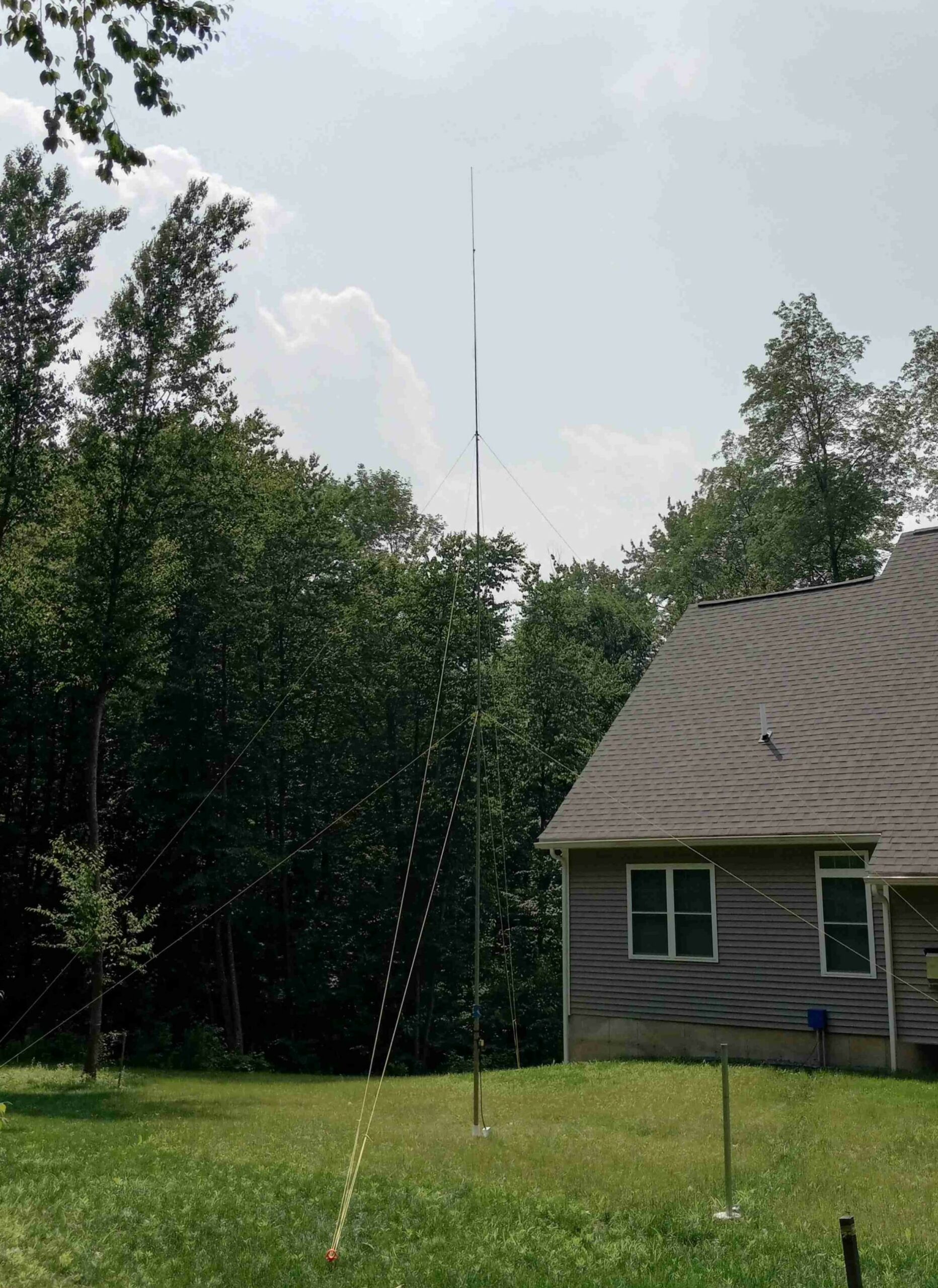
Figure 1. 20m L-Network Matched EFHW Vertical. The wire antenna and matching network is fastened to the fiberglass mast with rubber bongo ties. The mast height is 12.5m (41 ft). Base anchoring is accomplished with a hinged, tilt-over base mounting plate that was described in another article. Please click on the photo to enlarge it.
The antenna counterpoise consists of a 3 ft (~ 1m) section of outer coax shield, Figure 2. A line choke is inserted after this 3 ft section of coax to terminate the counterpoise. The remainder of coax to the shack is made up of a 40 ft long section of RG-8X.
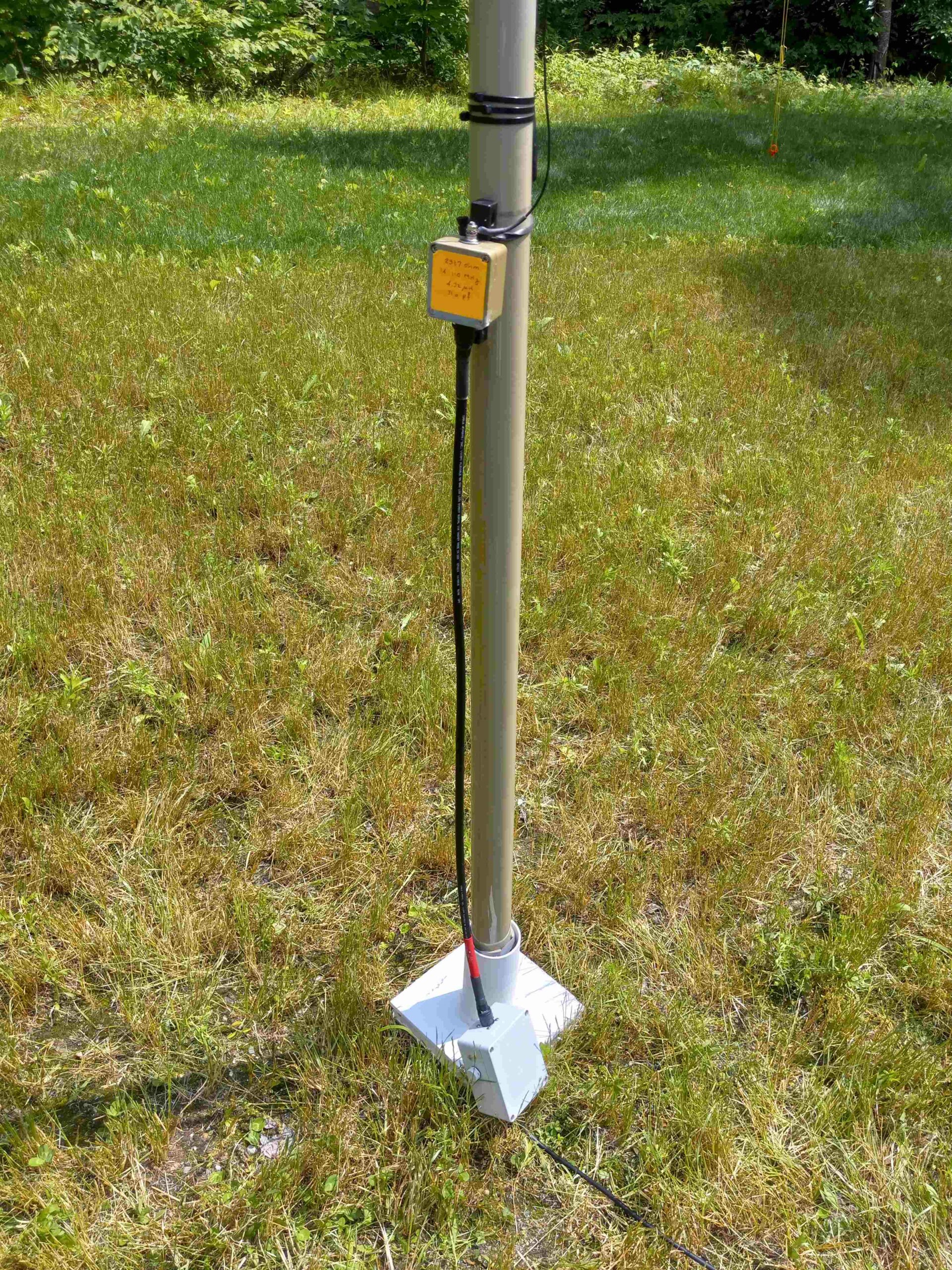 Figure 2. Matching Network, Coaxial Shield Counterpoise and Line Choke. The matching network was designed for 14.1 MHz. Since the matching network has a wide bandwidth, the antenna wire was cut slightly longer to resonate at the very bottom of the CW band. Please click on the photo to enlarge it.
A Smith Chart is plotted in Figure 3. It shows that the antenna match over the entire band is well within the 2:1 VSWR circle.
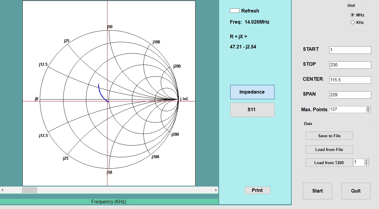 Figure 3. Smith Chart for 20m L-Matched EFHW Antenna. A match better than 2:1 match is achieved over the entire 20m band. The antenna wire was cut longer to provide the best match at 14.025 MHz. Please click on the photo to enlarge it.
The VSWR performance is plotted in Figure 4. The matching network consists of a lowpass L-network consisting of a series inductor followed by a shunt coaxial capacitor. The antenna wire has been cut to resonate at 14.025 MHz since I enjoy operating in the bottom 50 kHz of the 20m CW band. It’s not that the VSWR performance was that bad but I just could not understand why the antenna wasn’t achieving a near-perfect 1:1 match. I turns out that the residual mismatch is in the Polyphaser lightning arrestor located in the service entrance panel.
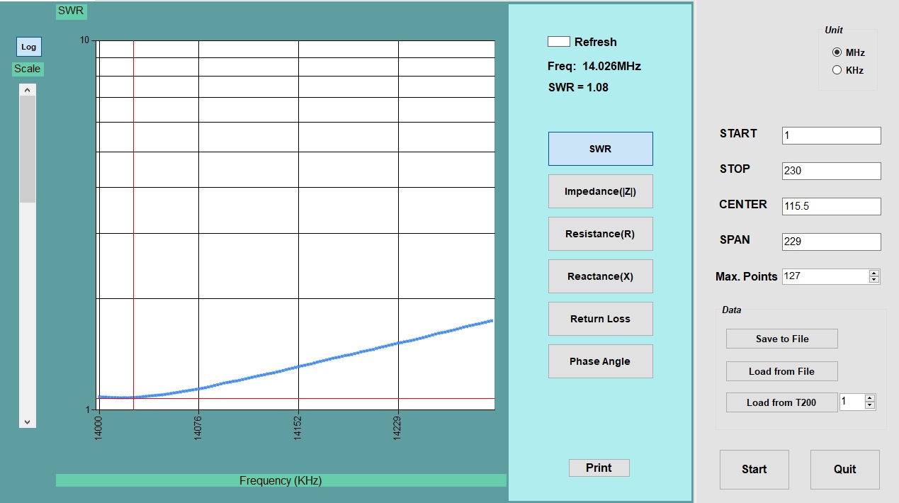 Figure 4. 20m VSWR Plot. The L-matching network exhibits wide bandwidth and good efficiency. The antenna wire is cut to resonate at the very bottom of the CW band where I like to operate. The match is very good but not perfect. This was due to the residual VSWR in the lightning arrestor located in the service entrance panel. Please click on the photo to enlarge it.
I operated a simple station consisting of an ICOM 718 at 100W to make three consecutive CW contacts with French stations. The next three days should produce some interesting DX.
References
[1] Blustine, Martin, Highly Efficient L-Matching Networks for End-Fed Half-Wave Antennas, June 11, 2022. https://www.n1fd.org/2022/06/11/l-matching-networks/
[2] Blustine, Martin, Tilt-Over Bases for Antenna Masts That You Can Build, June 30, 2022. https://www.n1fd.org/2022/06/30/tilt-over-bases/