Tag Archives: Mentor

Broadband Matching for Antennas

This article discusses some work on designing a matching network to make antennas match well (low VSWR) across the entire ham band.  This will be a described in more detail at the September Tech Night.

Antennas have an impedance (or match) that varies with frequency.   Transmitters want to see a matched antenna with an impedance of 50 ohms.    The antenna has the best match at one frequency and the match gets worse as the operating frequency changes.

Some bands and antennas are more challenging to match than others.  Shortened or loaded antennas have a narrow range of match frequencies.  The 75/80 meter band has a wide bandwidth in term of percentage.

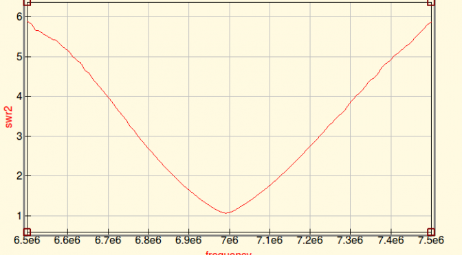
Here’s a plot of the SWR for my 40 Meter Dipole.  It’s a good match at 7.000 MHz and degrades to about 2:1 at 7.100 MHz.  Obviously, this is not optimized.

Broadband Matching - SWR for 40M Dipole
SWR for 40M Dipole

Modern radios have built in automatically adaptive matching networks make the radios work over a wider bandwidth, but networks are lossy and reduce transmitted power.

A manual antenna tuner has a lot lower loss than the built in tuner, but it requires manual adjustment.  In fact, the extra tuned circuits generally act to make the antenna have even less bandwidth.

The QUCS RF circuit simulation program has the ability to model SWR, bandwidth, matching networks based on data about antenna performance.  The antenna data can come from either an antenna modeling program such as 4NEC2 or EZNEC.  Or the data can come from a measurement made by a good antenna analyzer.

QUCS also has a built in optimizer.  It has the ability to try hundreds of circuit values and home in on an optimal design.

The optimizer setup needs a definition of “optimal”.  For the case of a broadband antenna, “The worst case SWR anywhere in the ham band shall be as low as possible”.  In the terms that QUCS understands, “minimize the maximum SWR over the frequency range 7.00 to 7.35 MHz.

Here is the result from running the optimizer on the data for my mistuned 40M dipole.  QUCS has designed a broadband matching network that can achieve less than 1.5:1 SWR over the whole band.

Broadband Matching

QUCS achieved this by varying the components of a filter network.  I drew a general filter network and let QUCS tune the component values.  This network is designed with coaxial stubs.

Broadband Matching

The model of the antenna is stored as a file in the X1 file component. Line7 is a 30-meter coax feedline.  The actual matching network consists of Line 1, 2, 3, 4.  Each line is 50 Ohm coax.  Line 1 and 3 are configured as open stubs.  The line lengths predicted by the model are…

  • Line 1: 7.75 meters
  • LIne 2: 4.47 meters
  • Line 3: 8.49 meters
  • Line 5: 8.03 meters

Here’s another example.  160-meter antennas are often implemented as shortened loaded verticals.  The loading makes the match very narrow-band.   The red curve in the plot below shows a top loaded 160 meter vertical.  It only covers a fraction of the band.Broadband Matching

The blue curve shows the result of an optimization run that selected the values for a 7 component matching network.  It achieves about 1.7:1 across the whole band.  This network uses capacitors and inductors because coax stubs would be very long on 160 meters.

Broadband Matching

The component values for this network…

  • C1: 3450 pF
  • L1: 3.954 uH
  • C2: 3978 pF
  • L2: 6.951 uH
  • C3: 6156 pF
  • L3: 2.831 uH
  • C4: 4778 pF

I have not built any of these networks to see how they work in practice.  The 160-meter network has some extreme values and it is probably very touchy to get right.  Building that network to handle Tx power will require vacuum variable capacitors in parallel with high quality stable fixed value capacitors.   But, the 160 network doesn’t really need 7 components.  Put in one less stage of L-C and the ripple across the passband goes up a bit.

Conclusions

QUCS is a great RF circuit simulator.  This shows that it can work with data from an antenna model or analyzer and can optimize matching networks to create a broadband antenna.

Jeff, WA1HCO

Hands-On Yagi Antenna Construction 2.0 for Teaching and Experimentation

The most important piece of equipment in ham radio is our antenna.  We are connected to the world with the magic of radio waves!  Each License Exam from Technician through Extra class has questions to test our knowledge on antenna design and building skills.  Home-brewed antennas are easy and relatively inexpensive projects.

This article describes a 2m, 3-element Yagi antenna construction concept that the N1FD FCC license teaching team has used over the last year for class demonstrations.  The “Lego” style construction (v. 2.0) shown in the above picture is our new design that demonstrates the operating principles of the ubiquitous basic dipole antenna as well as a 2-meter, 3 element Yagi.  (Note, This project evolved from an earlier effort by Diana Eng at Makezine.com, which can be seen here.

In this Newsletter issue, we will describe the construction of the “Lego” stylized antenna and show how it can illustrate basic properties of a dipole antenna.  We will build a Yagi antenna with the addition of reflector and director arms in a future Newsletter article.

CONSTRUCTION of the LEGO STYLIZED ANTENNA.

Yagi Antenna - Lego Antenna Parts and Receiver Antenna
Lego Antenna Parts and Receiver Antenna

The antenna demonstration unit consists of two assemblies. 

  1. A handheld receiver dipole set to a fixed frequency (e.g., 146.550 MHz). It is shown at the top of the photo above. It follows a “plumber’s delight” construction using pieces of PVC pipe for a short boom and handles.  The dipole arms are two telescoping (7-28 inch) FM radio replacement antennas, available on eBay or Radio Shack ($4-6 dollars).  The arms feed through the boom and are epoxied.  Bridging across the arms is a common 6-volt flashlight bulb.  The bulb lights up when the dipole receives a resonant rf signal.
  1. The “Lego stylized” Yagi antenna components are shown below the receiver unit. The boom (middle item) is made of red oak dimensioned at ¾  x  1 ½   x  48    The top surface is grooved to hold an epoxied  3/16  steel rod.  The bottom surface has drilled recesses to fit ¾ in PVC pipe for leg stands. The edge of the boom has two 24-inch adhesive tape rulers running from center to front and back of the boom.  The rulers read-out the spacing between the driven dipole element and the parasitic reflector and director arms. In the photo, the D.E. and parasitic elements are seen below the 48 in. boom.  The center element is the driven dipole and it is flanked by identical units that can be configured as either reflectors or directors.   Each unit consists of two telescoping FM radio antenna rods epoxied in a grooved piece of red oak ( ¾  x  1 ½  x  3 inches) serving as “riders” on the boom.  The telescope arms can be adjusted to “resonance” at any frequency in the 2-meter band. The bottom of all riders has 2 x ½ inch rare earth magnets.  These allow the three antenna elements to be fixed at any position on the 48 in. boom.

You can view a closer look at the assembled Yagi antenna configuration in this video (Click on Link)

DEMONSTRATIONS OF BASIC DIPOLE BEHAVIOR. 

1.  Antenna Resonance Determined by Dipole Length.

As we all know, the resonance length of a dipole is given by the equation:    L (in inches)  =  5616/ [ Frequency (in MHz)].  We can show this fact with aid of the “receiver” antenna, which is set for a frequency of 146.55 MHz  The light bulb of this antenna will light when it senses a signal of this value from our “Lego” antenna.

In the video below (Click on Link), we begin with a resonant D.E. length of 38.5 inches and see the receiver antenna light up.  Next, we manually shorten the D.E. and see the bulb light dramatically dim.  When the D.E. length is returned near the start value, the light bulb again brightens up.

  1. Effect of SWR on Signal Strength.

Most modern transceivers have a built-in auto-tuner that can match SWR up to 3:1.  We know this only makes the “radio happy”, still we key down without much thought on how our Tx signal degrades with a 3:1 match.  The pictures below use the transmitting “Lego” dipole and receiver dipole to show the received signals for an SWR of 1.1 and 3.0.  The SWR was changed by lengthening the D.E. elements by 2 inches while holding the Tx frequency at 146.55 MHz

Yagi Antenna - Receiver Signal-for Lego Dipole SWR 1.1
Receiver Signal-for Lego Dipole SWR 1.1
Yagi Antenna - Receiver Signal- for Lego Dipole SWR 3.0
Receiver Signal- for Lego Dipole SWR 3.0
3.  Polarization Effects between Tx and Rx Antennas.

A horizontal dipole shows “horizontal” polarization; meaning the electric field vector of the rf signal is parallel to the earth surface.  Similarly, a vertical dipole displays “vertical” polarization with the electric field perpendicular to the earth. We all learn this in a Technician class course.

When we use our 2m HT’s for short distance contacts, Tx and Rx antennas with opposite orientation create a huge signal loss.  The effect is shown dramatically in the video below.

CONCLUSION 

Our classroom constructible antenna for demonstrations in our Ham Radio license classes has evolved in design over the past year.  We believe it has been a useful resource,  helping students translate textbook theory to “Hands On” practice.  Perhaps, this review has kindled interest for our readers to think of their Next Antenna Project!

73 & Hope to hear you on the air,

Dave N1RF

Rig Audio Interfacing and Low Cost PC Headsets

First I want to promote some excellent papers on rig interfacing and grounding produced by Jim Brown K9YC.  There is a wealth of information there, produced by a very talented and experienced engineer.

Now…on to the topic of interfacing PC headset to ham rigs…

Heil Headsets get a lot of support and advertising in the amateur community.  But they are expensive.  The W2SZ VHF/UHF contest group that I belong to uses mostly Heil headsets, so I have a lot of experience with them.  The problem is that a lot of them are broken.  We only use them two weekends a year for about 36 hours but they fail in a variety of ways.

I don’t own a Heil headset (I’m too cheap), but wanted a more reliable headset for my own use on the mountain.  In this case, reliable means I can bring several for a reasonable price.  So, this led to a series of experiments with PC headsets that are available for prices that range from about $13 to $50.

PC headsets and Heil headsets operate differently.  Heil headsets use a dynamic microphone and cannot tolerate any DC current through the microphone.  PC headsets require a DC bias voltage to operate their electret microphone.

The diagrams below (copied from a great presentation on rig interfacing by AudioSystemGroup)  shows the two ways a PC puts electret bias on the ring terminal of the 3.5 mm microphone jack.

Rig Audio Interface Schematic

All PC headsets have the ring terminal for bias…that is the key to this design.

Rig Audio Interface Schematic

The box below takes 8 volts from the ICOM microphone connector and uses it to power the PC headset.  The circuit has…

  • 3.5 mm (1/8th inch phone) jack for the microphone
  • 0.47 uFd series cap on the microphone, pass audio and block DC
  • 2.2K resistor to pass DC from the 8V pin to the ring terminal
  • 1/4 inch phone jack for rig keying
  • Cable and ICOM microphone plug

Rig Audio Interface Circuit

Rig Audio Interface Circuit

It was important to ensure the Heil headset doesn’t see any DC if plugged into the microphone jack of this adapter.  The design put bias on the ring terminal to feed the PC headset.  But, the Heil microphone connector does not have a ring terminal so it simply grounds the bias voltage… so, no bias gets to the Heil.   The dynamic microphone in the Heil couples audio through the series cap.

Here’s another design.  This one has two 3.5 mm connectors, one jack, one plug plus a battery.  The battery supplies power to the PC headset without the need for power from the transceiver.  This also supplies power to the ring terminal and block DC to the microphone on the tip terminal.  This took about 5 minutes, the components are under the tape.

Rig Audio Interface Circuit

One of our W2SZ members, Tom Price KC2PSC, designed of a PC board to implement this idea.

  • RJ-45 connector for rig microphone interface
  • Converts to 3.5 mm microphone and line out
  • Converts 1/4 inch phone for rig keying
  • Includes option for battery

Rig Audio Interface Circuit

There are a number of web sites that discuss the same thing

Radio Amateurs Developing Skills Worldwide