Tag Archives: Antennas

Differential and Common Modes on Transmission Lines – Part II

Introduction

Differential and common modes on transmission lines were introduced in Part I [1] of this article. The use of baluns to mitigate common mode currents on transmission lines that feed dipole antennas were also discussed. Finally, the use and placement of common mode chokes were introduced.

In this installment, the work of Gustav Guanella [2] is chronicled, followed by Joe Reisert’s improvements [3] to Guanella’s original design. Next, the construction of a common mode choke is presented that includes data for the coax used. Finally, some analyses are performed to predict the performance of two common mode chokes, and graphical results are provided.

Guanella Balun

Gustav Guanella was a Swiss electrical engineer and prolific inventor. His name is associated with more than 200 patents [4]. One of his inventions was a new transformer design that appeared in The Brown Boveri Review in September 1944 [5]. Figure 1 depicts [6] his new transformer/coupler model. Two parallel, closely spaced wires are wound on an insulating core at a). The input and output center-tapped transformers at b) provide a means to separate and recombine differential and common mode currents in this embodiment. Differential, symmetrical currents (solid lines), i1, travel along a section of balanced transmission line at designation, A. Common Mode, asymmetrical currents (dotted lines), i2, travel along an alternate path through an RF choking inductor at designation, B.

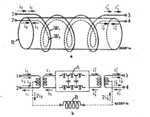
Figure 1. Guanella’s Double Wire Coil System with Equivalent Diagram. A two-wire transformer is wound on an insulating core at a). An equivalent circuit diagram is provided at b). The center-tapped transformers at b) provide a means to separate the differential current, i1, from the common mode current, i2. At A, the differential current passes through a balanced transmission line section, while at B, the common mode current is routed to a choking inductor. Reproduced with permission from ABB Ltd – The Brown Boveri Review, Vol. XXXI, No. 9, Sept. 1944, pp. 327 – 329, Baden, Switzerland.

Guanella’s simplest embodiment for a 1:1 balun is depicted in Figure 2 [7]. The inductance of the windings serves to suppress the asymmetrical (common mode) currents so that a balanced transmission line carrying symmetric currents in differential mode to the left may be connected to an unbalanced transmission line carrying asymmetric currents in common mode to the right. This transformation is possible regardless of frequency. Furthermore, Guanella demonstrates [8] that placing the inputs of more than one coil system in series on one side and in parallel on the other side can be used to implement transformations in the ratio of 1:N2 where N is the number of coil systems placed in series-parallel. For N=1, we have 1:12, which is just 1:1, as shown in Figure 2. An improvement to this design is presented in the next section.

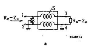
Figure 2. Guanella’s model for a 1:1 balun for transforming symmetrical balanced (differential mode) transmission line at the left to an unbalanced asymmetrical (common mode) transmission line to the right where one side is grounded. The suppression of the asymmetrical currents by the choking inductance of the windings makes it possible to connect balanced to unbalanced line. Reproduced with permission from ABB Ltd – The Brown Boveri Review, Vol. XXXI, No. 9, Sept. 1944, pp. 327 – 329, Baden, Switzerland.

Joe Reisert’s Improved Broadband Balun

Joe Reisert, W1JR, presented an interesting variation of the Guanella transformer in the September 1978 issue of Ham Radio magazine [9]. Unbalanced operation was described in Part I of this article which models the coax as a 3-wire transmission line. Symmetric differential mode currents will flow on the center conductor and inner shield, the desired mode of operation. However, there is nothing to prevent current from flowing on the outside of the coax shield since the outside and inside are conjoined at the antenna center insulator.

The Guanella design winds balanced wire transmission line on an insulating core, but there is no reason why an unbalanced coax cannot be wound on an insulating core to obtain a similar result. W1JR describes earlier versions of this design wound on ferrite rods [10]. In this configuration he states that there have been reports of “frequency sensitivity” over the decade in frequency required. There is also the problem of loss that will be a function of the magnetization admittance for the ferrite material chosen. Lower permeability materials will result in lower core losses but higher flux leakage. Rods will result in higher flux leakage than a toroid. Lower permeability cores will require more turns to achieve the same impedance as toroids for similar materials. Now that #31 with initial permeability, μi, of 1500 and #43 material with initial permeability, μi, of 800 are available, they are logical choices for HF use. The impedances of the windings will vary as a function of frequency, but 11 or 12 turns on these cores are adequate to provide a great deal of common mode attenuation over the HF frequency range. The core losses as a function of the number turns on toroid ferrite cores were the subject of an earlier article [11].

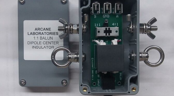
Figure 3 illustrates W1JR’s improved design [12]. This device is suitable for use as an antenna balun as illustrated. When both ports are terminated with coaxial connectors, the device is suitable for use as a common mode choke. To paraphrase the Traub Manufacturing Company slogan [13], Joe Reisert’s balun is “Often imitated, frequently duplicated.”

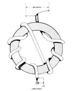
Figure 3. W1JR’s Improved Broadband Balun. Eight turns are depicted in this graphic. Since the crossover winding passes through the core, it counts as a single turn. This 1:1 balun will transform unbalanced coaxial transmission line to the balanced feed point of a dipole antenna. If the balanced side is connectorized, the balun becomes a common mode choke. If sufficient inductance is present for the outer coax shield, the asymmetric common mode currents on the outer coax shield are suppressed. Reprinted with permission from the September 1978 issue of Ham Radio magazine, © CQ Communications, Inc.

Fabrication

Coax Properties

Two coaxial cable types under consideration for common mode choke fabrication are RG-303/U [14] and RG-400/U [15].

Voltage Specifications

We consider RG-303/U that was recommended in Joe Reisert’s article [16] and RG-400/U that was used in the construction of two common mode chokes described in this article. Both are compact PTFE coaxial cables characterized by working voltages of 1400V RMS, or 1980V peak. Assuming that the cables are perfectly matched to the transmitter and the antenna, the peak voltages on the cables are found to be,

where:

P0 is the transmitter power – for example 1500W

Z0 is the characteristic impedance of the coaxial cable, 50 ohms

Thus,

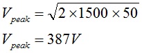
The peak voltage on the line for a matched system is 387 volts for 1500W. This does not challenge the voltage specification of the coaxial cable.

Next, let’s consider the case where the antenna is mismatched to the line. As an example, a 6:1 VSWR will be considered. For this case the magnitude of the maximum peak voltage on the transmission line may be as great as [17],

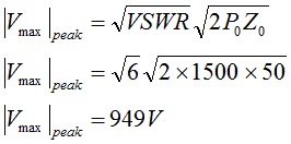
This voltage is well within the specification limits for both coaxial cable types with the proviso that the connectors have been properly installed on the cable ends.

Minimum Coaxial Cable Bend Radius

The bend radius of the coaxial cables should be considered for both cable types. For RG-303/U the minimum bend radius [18] is specified to be 2” (50.8mm) while for RG-400/U a value of 1” (25.4mm) applies [19]. Because of the sharp bends required around the stacked FT240 toroidal ferrite cores during the winding process, it would appear that neither coax meets the bend radius requirement. Since Teflon will deform, it is expected that, over time, the center conductor will migrate from the center of the dielectric.

Power Handling Capability

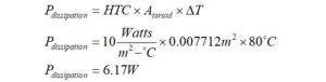
This discussion would not be complete without a few words about the power handling capability for the ferrite used. The #31 and #43 ferrite materials possess high permeability properties. They are also lossy.

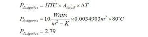
A discussion of power handling capability for ferrites was provided in a previous article [20]. This topic may not be ignored for ferrite use at high power. The higher the permeability, the more lossy the material will be. Of the two materials cited in this article, #31 with an initial permeability of 1500 has the highest loss. It is absolutely essential that the choking impedance be as high as possible and that the material loss be as low as possible to prevent overheating. PTFE coax is unlikely to melt, but ferrite cores have been known to shatter due to thermal runaway once the Curie temperature is reached. This is a safety concern. Contrary to what has been written on the web, ferrite devices used in power applications should always be enclosed and properly ventilated if required.

The heating effect is due to the outer shield being wrapped around the ferrite core which has a choking effect. The inner coax transmission line operating in differential mode by itself is not the cause of heating. The outer coax shield must be treated as a third common mode transmission line from a standpoint of dissipative loss when wrapped around the core.

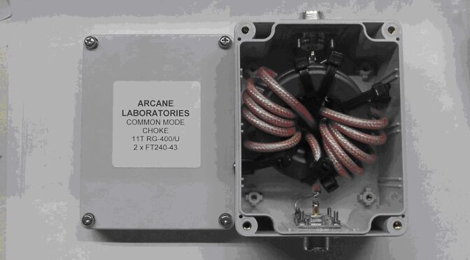
Construction Details

Seven connectorized common mode chokes were constructed for use in transmission lines and for use at the operating location, as required. Without line chokes common mode currents are apt to find their way back to the operating location on the coax shield. Common mode currents can create reception, equipment and operator problems. For maximum effect the choking impedance should be located at a voltage node in the transmission line where the wave impedance of the standing wave is low [21]. If a dipole antenna is in use, a choking balun should also be located at the feed point.

The line chokes were constructed on stacked cores of FT240-31 and FT240-43 material. The literature recommends both for EMI suppression [22]. Eleven turns of RG-400/U coax were wound on each of the stacked cores with a Joe Reisert, W1JR, crossover winding in the center. Each choke was housed in a Bud Industries PN-1323 box [23]. Holes were drilled in the housings with a Milwaukee step drill [24]. Step drills are essential for boring holes in plastics and metals, and they are well worth the initial investment. Connections are made to the coax shield using the technique best illustrated in Figure 4. A short length of insulation is removed from the coax, the coax braid is tinned and the short piece of buss wire is wrapped around the braid and soldered. If PTFE coax is used, nothing will melt. The free end of the buss wire is bonded to the UHF connector flange with a solder lug and #4-40 hardware. The buss wire should be as short as is practical.

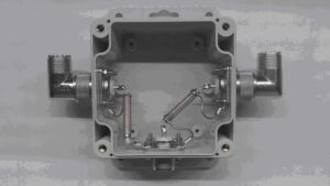
Figure 4. Connecting to the Coax Shield. The recommended method for connecting to the coaxial shield is pictured. Since the dielectric is PTFE, it will not melt when the braid is tinned. Where required, a short length of shrink tubing may be used to cover the exposed shield.

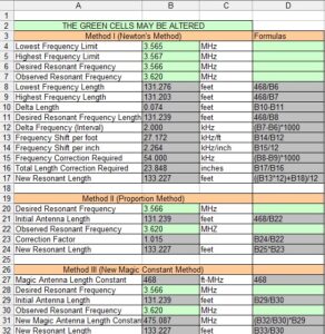
Common Mode Choking Impedance Predictions

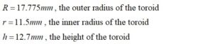
Common mode choking impedances were estimated for stacked cores consisting of 2 x FT240-31 and 2 x FT240-43 ferrite toroid materials. Eleven turns of RG-400.U were wound on each stacked core. The choking impedance for each was calculated as a function of frequency for each core. Permeability data was obtained as a .csv file for each core at the Fair Rite website.

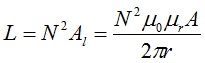
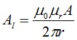
Since the inductance of a toroid is calculated from the value of the magnetic flux by the expression,
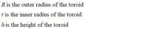
where:

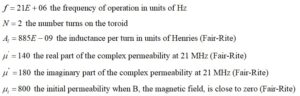
N is the number of turns wound

Al is the inductance per turn in units of Henries, H

μ0 = 4π x 1E-07 is the permeability of free space in units of H/m

μr is the relative permeability constant, dimensionless (relative to μ0)

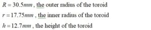
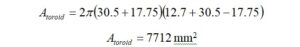
A is the cross-sectional area of the core in units of m2

r is the average radius of the core in units of m.

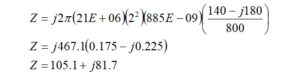
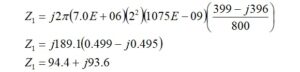
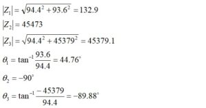
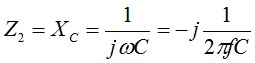
the complex impedance may be calculated from,

where:

L is the inductance in units of Henries, H

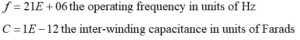
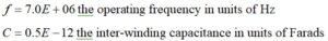
ω = 2πf the angular frequency in units of radians/s

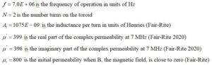
f is the frequency of operation in units of Hertz, Hz, or s-1

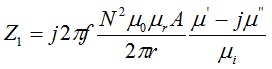
Since the value of Al is based upon the value of μi, the initial permeability at 10 kHz, the permeability value must be modified to include the complex permeability. This is key to deriving the frequency dependence of impedance based upon the complex permeability [25].

Thus, we may write:

where:

μi is the initial permeability, dimensionless

μ’ is the real part of the complex permeability, dimensionless

μ” is the imaginary part of the complex permeability, dimensionless

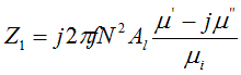
If the value of Al happens to be provided by the ferrite manufacturer, the expression for Z is simplified to,

If the value of Al is not readily available, it may be calculated from,

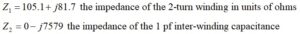
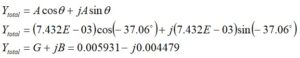
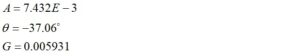
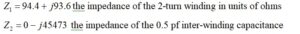
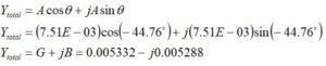
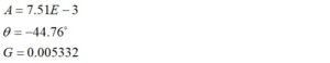
A value, 2 pf, for an interwinding capacitance was incorporated into the calculation by placing it in parallel with the toroid winding. It’s a guess. Recall that,

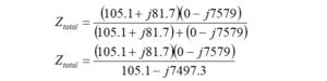
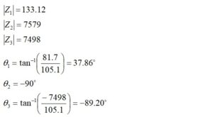
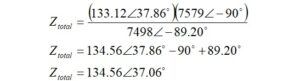
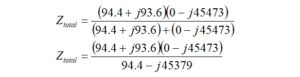
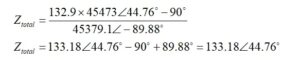
Applying the formula for parallel impedances,

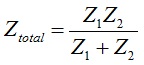
the choking impedances were plotted for 11 turns on 2 x FT240-31 and 2 x FT240-43 stacked ferrite toroid cores. The calculations are quite tedious, so some automation is essential. An Excel spreadsheet can be generated after .csv files have been downloaded with frequency-dependent, complex permeability data from the manufacturer, Fair Rite. The results appear in Figures 5 and 6, respectively. Depending upon the provenance of the ferrite used, actual results may vary by ± 20%.

If a nanoVNA is available, the impedance of the outer shield winding may be measured. Then, the resonant frequency of the common mode choke, which is the zero crossing of the reactance, may be determined. These points are visible in Figures 5 and 6 at 6.2 and 7 MHz, respectively. Once the resonant frequency has been determined through measurement, the capacitance value in the analysis for Z2 can be adjusted so that the frequency of resonance for the analysis data matches the measured data.

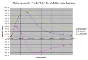
Figure 5. Choking Impedance for Stacked FT240-31 Cores. Eleven turns were modeled on 2 x FT240-31 cores. A 2 pf capacitor is modeled in parallel with the winding to represent the interwinding capacitance. The choking impedance is sensitive to the number of turns and an interwinding capacitance that tends to reduce the impedance with increasing frequency.

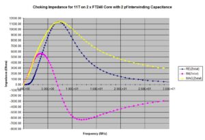
Figure 6. Choking Impedance for Stacked FT240-43 Cores. Eleven turns were modeled on 2 x FT240-31 cores. A 2 pf capacitor is modeled in parallel with the winding to represent the interwinding capacitance. The choking impedance is sensitive to the number of turns and an interwinding capacitance that tends to reduce the impedance with increasing frequency.

Performance measurements for the common mode chokes described in this article are presented in Part III.

References

[1] Martin Blustine, K1FQL, Differential and Common Modes on Transmission Lines – Part I, July 25, 2022. https://www.n1fd.org/?s=Common+Mode
[2] Biography, Gustav Guanella, Wikipedia, https://en.wikipedia.org/wiki/Gustav_Guanella
[3] Joe Reisert, Simple and Efficient Broadband Balun, Ham Radio, September 1978, pp. 12 – 15.
[4] Biography, Gustav Guanella, op. cit. https://en.wikipedia.org/wiki/Gustav_Guanella
[5] Gustav Guanella, New Method of Impedance Matching in Radio-Frequency Circuits, The Brown Boveri Review, V. XXXI, No. 9. pp. 327 –329. https://library.e.abb.com/public/dadf14b477e54194ba7613a3aae11e7a/bbc_mitteilungen_1944_e_09.pdf?x-sign=lWb6zmbVjwsVidyeEEIqKcRGbQm7nu2SHtvRAO9177wOzUNw0KaE8CNmiu5MYIfM
[6] Ibid, p. 327.
[7] Gustav Guanella, op. cit., p. 328.
[8] Gustav Guanella, op. cit., p. 328.
[9] Joe Reisert, op. cit.
[10] Joe Reisert, op. cit., p. 13.
[11] Martin Blustine, K1FQL, Power Losses and Dissipation in Various Ferrite Devices – Part II, August 12, 2022. https://www.n1fd.org/2022/08/12/ferrite-loss-2/
[12] Joe Reisert, op. cit., p. 13.
[13] Traub Manufacturing, https://www.quora.com/Who-coined-the-phrase-Often-imitated-never-duplicated
[14] Belden RG-303/U, https://catalog.belden.com/index.cfm?event=pd&p=PF_84303
[15] Belden RG-400/U, https://edesk.belden.com/products/techdata/EUR/MRG400.pdf
[16] Joe Reisert, op. cit., p. 14.
[17] Martin Blustine, K1FQL, Worst Case Standing Wave Voltage on a Transmission Line, August 1, 2022. https://www.n1fd.org/2022/08/01/standing-wave-voltage/
[18] Belden RG-303/U, op. cit.
[19] Belden RG-400/U, op. cit.
[20] Martin Blustine, K1FQL, Power Losses and Dissipation in Various Ferrite Devices – Part II, op. cit. https://www.n1fd.org/2022/08/12/ferrite-loss-2/
[21] Chuck Counselman, W1HIS, Common-Mode Chokes, YCCC, April 6, 2006, p.13. https://remoteqth.com/img/ZAW-WIKI/cmcc/CommonModeChokesW1HIS.pdf
[22] https://www.fair-rite.com/product-category/suppression-components/round-cable-emi-suppression-cores/
[23] https://www.budind.com/product/nema-ip-rated-boxes/pn-series-nema-box/ip65-nema-4x-box-pn-1323/ – group=series-products&external_dimension
[24] https://www.homedepot.com/b/Tools-Power-Tool-Accessories-Drill-Bits/Milwaukee/Step/N-5yc1vZc248ZzvZ1z0y9ih
[25] Owen Duffy, VK1OD, A Method for Estimating the Impedance of a Ferrite
Cored Toroidal Inductor at RF, December 29, 2015.
https://owenduffy.net/files/EstimateZFerriteToroidInductor.pdf

How to Prune A Dipole Antenna to Length

Introduction

Whether it is for a half-wave dipole or an end-fed half-wave antenna, sooner or later we will have to prune one of these antennas to the correct length. Most of us are accustomed to trial-end error when it comes to tuning a dipole, but there are better ways to do it [1]. This paper describes three methods for your consideration. All of the formulas for the techniques shown may be entered into an Excel spreadsheet. If you do not have Excel on your computer and you have access to Google, you can use Google Sheets [2]. If you have Windows on your computer and have registered, then you can log into your Windows account and use Excel for free at office.com [3]. All three computation methods described may be entered onto a single spreadsheet, as in Figure 1, or entered onto separate tabs.  All three techniques will produce the same answers. Most everyone owns a smartphone, so you can bring your spreadsheet app to the yard with you.

Directions for Loading the Spreadsheet

Figure 1 lists the spreadsheet formulas in Column D.  Type these formulas over into Column B. Begin typing in Row 8, Column B. You must type an equal sign in front of every formula for the sheet to work. Once the formulas have been entered, enter the variables in the green cells in Column B. It is a good idea to lock the gray cells to protect the formulas from being over-typed.  Then, protect the entire sheet so that the only cells open for data entry will be the green cells in Column B. If you click on Figure 1, it will open into a new window for easier viewing.

Figure 1. Sample Spreadsheet. Any one of the three methods or all three may be entered onto a single spreadsheet, or onto multiple spreadsheet tabs. A spreadsheet app on your smartphone is an easy way to carry the calculator to the field.

Descriptions of the Methods Used

Method I – Newton’s Method

The first method is one invented by Isaac Newton, but not for antennas. Newton was working with what we now call differential calculus in the late 17th century, which helps to put his genius into perspective. These days, we learn this technique in the first few weeks of calculus in high school. If we use the familiar formula to calculate the length of the dipole at a frequency just above and just below the desired frequency we can get a frequency differential.

If we subtract the two lengths, we get a length differential. By dividing the frequency differential by the length differential, we arrive at the number of kHz the resonant frequency moves per unit of length pruned. If we choose a very narrow frequency interval around our desired frequency, this technique becomes very precise. It’s a kind of sensitivity analysis. We move something a little bit and something else changes a little bit. That’s a hint as to what calculus is all about.

Method II – Proportional Method

The second method, which we call the proportion method, uses the familiar dipole length formula to arrive at the dipole length at a design frequency. In the field, we measure the frequency at which the antenna actually resonates. If we divide the observed frequency by the desired frequency, we arrive at a correction factor by which we multiply the old length to get the new length.

This is the most commonly used method for pruning an antenna.

Method III – New Magic Constant Method

The third and last method is called the “magic constant” method. We all remember that we divide 468 by the frequency in MHz to arrive at the dipole length in feet. The number 468 is what we call the “magic constant.” Suppose we calculate the length of a dipole using the magic constant. In the field, we observe that the dipole resonates at a different frequency. If we divide the observed frequency by the desired frequency, we arrive at a correction factor that can be multiplied by the old magic constant to get a new magic constant.

Then, we use this new magic constant to calculate a new antenna length.

Of the three methods, only the first method is a bit arcane because it uses differential analysis. The latter two are equivalent because they use proportions.

References

  1. https://www.hamuniverse.com/easydipole.html
  2. https://www.google.com/sheets/about/
  3. https://www.office.com/

Power Losses and Dissipation in Various Ferrite Devices – Part II

Introduction

In Part I, the magnetization admittance [1] was employed to calculate the fractional power lost to an FT140-43 ferrite core by a 10-turn winding at 21 MHz [2]. Part II will show how to calculate the amount of power the same ferrite core can dissipate into free air before reaching its Curie temperature. Modulation methods and duty factors will be figured into these calculations. Whether it is an inductor, transformer, or balun, the analysis is similar.

Although the maximum permissible ferrite temperature will not change as a function of the transmitting mode used, the maximum permissible amount of input transmitter power will. This subject will be explored in the context of ferrite transformers, including one sold by the ARRL for use in an end-fed half-wave antenna kit.

Recap

By way of review, it was shown in Part I that the percentage power lost to the ferrite core described in the introduction is given by,

where:

The amount of power lost to the core is 1.18%.

While this is useful to know, we would also like to be able to calculate the amount of power that may be dissipated by the ferrite core to free air before the Curie temperature is reached. The Curie temperature is the temperature at which there are drastic changes in the material’s ferrimagnetic (Ferri, not Ferro) properties. When ferrite is used in the construction of antenna components, the Curie temperature will dictate what our transmitter operating power can be for specific modes and duty factors of operation.

Ferrite Core Efficiency

From the core loss, we may now calculate the efficiency from the expression,

This sounds like good efficiency, but it doesn’t take many Watts in a confined space to heat ferrite above its Curie temperature as will be shown.

The core loss in dB is calculated from the expression,

Maximum Long-Term Average Power Dissipation

Case I

Next, we find the Curie temperature for #43 ferrite material from the datasheet [3],

We now consider the ambient operating temperature. For outdoor use in the summer, the ambient temperature inside an enclosure can easily rise to 50⁰C, and this may well be on the low side. It can easily be that hot in an attic during the summer.

If we take the Curie temperature and the ambient temperature into account, the allowable ferrite temperature rise is,

Next, we need to find a value for the convective heat transfer coefficient (HTC) for the ferrite into free air. The value offered by Owen Duffy [4] is,

This number appears in another paper [5] published by the U.S. Army Research Laboratory for ferrite subject to natural convection of 0.5 m/s, although 14 Watts/m2-K appears to be an upper limit.

Surface Area of a Toroid Core

Next, we need to calculate the surface area of the ferrite toroid of a rectangular cross-section using the formula,

derived from the geometry of a hollow cylinder,

where:

Expanding the difference of squares and collecting terms obtains the simplified expression,

For an FT140-43 ferrite core, the dimensions are [6],

Recalling that 1 mm2 = 1E-6 m2

This area does not correct for any bevels or radii on the edges of the ferrite core.

The maximum long-term average power dissipation in Watts is given by,

The maximum long-term average power dissipation is 2.79 Watts. This may come as a surprise, but that is all that it takes to cook this ferrite core if it is housed in a sealed box. At this point, it may be appropriate to advise that ferrite should be enclosed when subjected to even moderate amounts of power. Ferrite has been known to explode into shards. If more ventilation is required, enclosure manufacturers like Bud Industries make baffled vents for their enclosures. Some ferrite transformer manufacturers have recognized that vents should be added to their product lines.

Next, we need to calculate the maximum continuous average RF power in Watts that can be applied, which will result in a power dissipation of 2.79 Watts. This is given by the expression,

where:

The maximum continuous average RF power that can be applied is 236.4 Watts.

Apparently, 10-turns on an FT140-43 core at 21 MHz is very efficient. That is due to the number of windings on the core, which tends to reduce flux leakage.

Case II

Next, we reduce the number of turns on the ferrite core to 2-turns, as is very often the case for transformer primary windings used to match end-fed half-wave antennas. Ultimately, we will need to calculate the value of conductance, G, for the new winding configuration at 21 MHz so that we may repeat the calculations.

We start by calculating the impedance for the new configuration [7],

where:

The impedance for a 2-turn transformer primary winding is 105.1+j81.7 ohms. We would like to place a 1 pf inter-winding capacitance in parallel with the primary impedance.

The capacitive reactance is calculated from,

where:

The capacitive reactance that will be in parallel with the impedance is 7579 ohms.

We calculate the parallel combination of two impedances using the formula

where:

We could rationalize the denominator and simplify or convert it to polar form.

Let’s convert the impedances to polar form to arrive at the parallel combination. We define a new impedance for the denominator, Z3.

The capacitor has a phase angle θ2 = -90⁰ because the voltage lags the current.

Now, we construct Ztotal in polar form,

This is easily converted to admittance,

Note that the sign of the angle changes when it is moved to the numerator.

Converting back to rectangular form with the help of the Euler identity provides what is needed,

where:

Once again, we calculate the power lost to the core,

Reducing the number of turns on the core has resulted in an enormous core loss.

The efficiency may be calculated,

The core loss in dB is,

The core loss is 1.53 dB.

The maximum long-term average power dissipation for the core does not change. It remains 2.79 Watts.

Now, we calculate the maximum continuous average RF power in Watts that can be applied which will result in long-term average power dissipation of 2.79 Watts.

The maximum continuous average RF power may not exceed 9.39 Watts.

Apparently, 2-turns on an FT140-43 core at 21 MHz is not very efficient. If we were to consider CW operation at a duty factor of 44%, we might be able to apply,

QRP operation on CW at 21 MHz should not be a problem.

For SSB that operates at an average power of about 10% PEP/Pavg, 93.9 Watts might be possible without overheating. This is a conservative number that includes speech compression. For uncompressed speech operating at 3% PEP/Pavg, 313 Watts might be possible.

Case III

Let’s analyze the case of the ARRL End-Fed Half-Wave Antenna Kit. The specifications state that this antenna is rated at 250 Watts PEP. The core used in the kit is an FT240-43. The turn ratio is 2:14 (1:7) for an impedance transformation of 1:49. The transformer is intended to match a 50-ohm source to a 2450 ohm load. The voltage requirement for the compensation capacitor in the kit will also be included in this analysis. Let’s assume operation at the very bottom of the 40m band, 7.0 MHz.

Surface Area of the Core

For an FT240-43 ferrite core, the dimensions are,


Recalling that 1 mm2 = 1E-6 m2

This area does not correct for any bevels or radii on the edges of the ferrite core.

Maximum Long-Term Average Power Dissipation

The maximum long-term average power dissipation in Watts is given by,

The larger FT240 core is capable of higher power dissipation before reaching the Curie temperature.

Primary Winding Impedance and Admittance

In order to calculate the efficiency of the FT240-43 core with 2 primary turns, the admittance will be required at 7 MHz. As before, we first calculate the impedance from the expression,

where:

The impedance for a 2-turn transformer primary winding is 94.4+j93.6 ohms. We would like to place a 0.5 pf inter-winding capacitance in parallel with the primary impedance.

The capacitive reactance is calculated from

where:

The capacitive reactance that will be in parallel with the impedance is 45473 ohms. Thus, the impedance of the inter-winding capacitance is,

We calculate the parallel combination of two impedances using the formula,

where:

Again, we could rationalize the denominator by multiplying the top and bottom by the complex conjugate of the denominator or convert the top and bottom to polar form. Let’s convert to polar form and solve. We can assign impedance, Z3, to the denominator that has already been simplified.

Thus,

Please note that when the angle is moved from the denominator to the numerator, there is a sign change. We need the total admittance, and that is easy to calculate from,

Next, we convert the total admittance to rectangular form to recover the value of the conductance, G.

Converting back to rectangular form provides what is needed,

where:

Power Lost to the Core

Once again, we calculate the power lost to the core from,

The magnetization admittance loss is substantial at 7 MHz.

Core Efficiency

The efficiency may be calculated from,

Core Loss

The core loss in dB is,


The core loss is 1.38 dB.

Maximum Continuous Average RF Power

The maximum long-term average power dissipation for the core does not change. It remains 6.17 Watts.

Now, we calculate the maximum continuous average RF power in Watts that can be applied, which will result in a power dissipation of 6.17 Watts.

The maximum continuous average RF power may not exceed 23.1 Watts.

CW Operation

Apparently, 2-turns on an FT240-43 core at 7 MHz is not very efficient. If we were to consider CW operation at a duty factor of 44%, we might be able to apply,

QRP operation on CW at 7 MHz should not be a problem, but 100W CW operation would be a problem for a long tune-up and long-winded QSOs.

Uncompressed SSB operates at a 3% PEP/Pavg ratio [8], and that mode should be no problem at all for up to 769 Watts. Even in compressed audio operation at a 10% PEP/Pavg ratio [9], 231 Watts should not be an issue.

If we revisit everything in terms of Intermittent Commercial and Amateur Service (ICAS), everything changes. We find that the maximum continuous RF power becomes 46.2 Watts. CW operation becomes possible for up to 105 Watts. Uncompressed SSB operation is possible for up to 1538 Watts, and compressed SSB is possible for up to 462 Watts.

SSB looks like a success, while CW looks a bit marginal for all but short-duty QSOs during summer temperatures. At least for CW, operating habits contribute to success or failure.

Compensation Capacitor Voltage Rating

Next, let’s look at the capacitor used in the kit.

The ARRL kit is supplied with a compensation capacitor to be added to the transformer input. The instructions state that this capacitor may be omitted unless operation is required on the higher bands. It would be useful to know what its voltage rating should be under conditions of elevated VSWR [10]. The parts list tells us that the value of the capacitor is 100 pf and the voltage rating is 2 kV. This information is in the parts list. We are not told what the dielectric characteristics of the capacitor are.

If we assume operation in a system where the antenna mismatch is as bad as 6:1, we can calculate the maximum peak voltage on the transmission line that connects to the transformer input. The capacitor shunts the input. The calculations are performed for a 100 Watt transmitter.

Previously [11], it was demonstrated that the maximum peak voltage on a transmission line may be calculated from,

where:

VSWR is the voltage standing wave ratio on the transmission line

P0 is the power incident on the transformer, 100 Watts

Z0 is the characteristic impedance of the line, 50 ohms

If we assume a 6:1 VSWR, we can calculate the maximum peak voltage as,

If a 500 V capacitor were used, there would be more than 100% margin. The 2kV capacitor that is furnished with the kit far exceeds what is required.

Compensation Capacitor Dielectric Dissipation

It would also be useful to know how much dissipation there is in the capacitor. Poor quality ceramic capacitors possessing low Q can easily overheat.

Calculation of Q for a Capacitor

First, the magnitude of capacitive reactance at the desired operating frequency is calculated.

where:

For example, the value of Xc is calculated at 7 MHz for a 100 pf compensating capacitor. The capacitive reactance at 7 MHz for a 100 pf capacitor is,

Next, the equivalent series resistance (ESR) of a capacitor may be calculated from the capacitive reactance and the dissipation factor,

where:

A typical Class III ceramic capacitor of 100 pf has a dissipation factor of 0.05 (5%) at 1 MHz, while a typical silvered mica capacitor has a dissipation factor of 0.00075 (0.075%) at 1 MHz. The dissipation factor does not change rapidly with frequency.

The ESR and Q for the Class III capacitor is calculated at 7 MHz,

where:

Q is the capacitor quality factor, dimensionless

Similarly, if the ESR and Q are calculated for a silvered mica capacitor at 7 MHz,

The lowest dissipation factor occurs for the silvered mica capacitor at 7 MHz as compared to the Class III ceramic capacitor.

Calculation of Dielectric Power Dissipation

In order to calculate the power dissipation for each type of capacitor, the equivalent shunt loss resistance is required,

For the ceramic capacitor, we obtain,

We repeat for the silvered mica capacitor,

The RMS voltage for 100 Watts into 50 ohms is given by,

The dissipations are for the ceramic capacitor,

and for the silvered mica capacitor,

It appears that a Class III capacitor is apt to cook if used as the compensation capacitor, while silvered mica parts might be a better choice. Better quality Class I ceramic and silvered mica capacitors with low dissipation factors are readily available.


Radio Amateurs Developing Skills Worldwide