Getting Started with POTA and Portable Operation

Background

The Nashua Area Radio Society (NARS) leadership saw that there may be a lot of latent interest in Parks On The Air (POTA) and portable HF radio operation but club POTA events were not very well attended.  Some members had noted that they would like to get involved with POTA but didn’t know how to start.  Not knowing about portable operation and not necessarily having the right equipment, folks were reluctant to attend a POTA event.  The leadership decided to kick off a “Tiger Team” of interested members in the summer of 2023 to concentrate knowledge in this type of radio operations and share it with all interested members.  The team has set the following goals:

  • Build and improve the skills needed for successful portable operation
  • Share this knowledge in one or more POTA events open to all club members, even those with no equipment of their own and/or no portable operation experience, providing a hands-on opportunity for inexperienced members to learn about and experience POTA operation in a no-stress environment
  • Promote continued interest in POTA and SOTA through the next year

A Tiger Team is loosely defined as “a group of experts brought together to solve a specific problem”. A number of members volunteered for this team, with a core group of eight consistently contributing to the effort. Interestingly, while a few of these volunteers had some POTA operating experience, more than half had little or no experience but were very interesting in learning this skill.

Learning

The team  started by identifying learning resources, and we found a number of promising sources of information including:

  • ARRL Courses
    • Getting Started with Parks On The Air
    • Getting Started with Summits On The Air (SOTA)
  • pota.app and sota.org.uk websites
  • NARS Tech Night presentations and Articles
  • YouTube instructional videos (search for POTA or SOTA)
  • Books
    • Portable Operating for Amateur Radio, ARRL
    • The Parks on the Air Book, ARRL (new)

There were two areas of learning that we pursued:

Portable Operation

The equipment and operating techniques used for base stations are similar to those required for portable operation, but portable operation comes with its own unique challenges including

  • Smaller and more rugged radios
  • Low Power (QRP) operation
  • Antenna options suitable to each particular location of the activation, as well as the ability to quickly assess the site, erect the appropriate antenna, and tune it for the band(s) being used in the activation.
  • Power supplies that are “off the grid”, easy to carry, and with enough capacity to allow operation for the duration of the activation (which could be for a day or several days depending on the trip.)
  • Ability to carry in, set up quickly and easily tear down and carry out, in order to maximize the time available for radio operation.
  • Being well organized with equipment that is easy to pack and transport.

Parks On The Air Procedures

There are particular procedures for the operation, logging, and reporting in order for operation to be considered a POTA activation.  For example, how to identify the particular state or national park or parks being activated using coded designations,  what information to exchange over-the-air, and how to report logged contacts.

Practice Outings

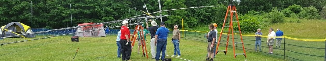
Armed with this information, team members then held a number of practice POTA outings at local parks including Miller State Park (K-2662) on Pack Monadnock, Rollins State Park (K-2676) on Kearsarge Mountain (K-4918), and Litchfield State Forest (K-4922), all in New Hampshire. During these outings, the experienced members “Elmer”ed while everyone experimented and learned. The team then identified available equipment and planned the an “Enhanced POTA” club event to take place on October 15th. At this event, all club members were invited to attend regardless of skill levels or equipment owned, and were promised the opportunity to operate just as in the annual Field Day.

Setting for the Enhanced POTA Event

The team chose Winslow State Park (K-2685) in the Kearsarge Mountain State Forest (K4918) for the event. Being at a park within a park made this a “POTA dual activation”. Winslow State Park is situated at 555 meters (1,820 feet) elevation on the northwest slope of Kearsarge Mountain, some 340 meters (1,117 feet) below the summit.

POTA
Winslow State Park View to the West

The park has a covered pavilion at the edge of a flat open area, with a number of nice trees nearby for the erection of wire antennas.  Conveniently, this area was only a short walk from the parking area, making it easy to carry in equipment.

POTA
Pavilion

The day was dry but cloudy and cool with a steady breeze, making for a chilly day of operation. Nevertheless, spirits were high among the twelve members of the Nashua Area Radio Society who participated, along with a number of visitors who stopped by to see what was going on (including a park ranger).

Motivation

Participants shared a number of reasons they found Portable/POTA operation interesting and fun, including:

  • Combining love of ham radio with enjoyment of the outdoors
  • Meeting the challenges of portable operation, including assembling and organizing gear, practicing antenna setup skills at a variety of sites, and addressing other limitations including portable power and QRP operation.
  • Portable operation forces you to work through “the basics” with every activation.
  • Enjoying the comradery of other portable operators
  • Hams who are not able to set up a home base station are able to operate an HF station
  • It’s like a Field Day operation every weekend

Stations

We had a total of five stations operating on five bands (40m, 30m, 20m, 15m, and 10m) using several modes including SSB, CW, and FT8. This provided a nice variety of radios, antenna styles, and power sources for operation during the event.

40 Meters

Ed KA6PNL arrived early in the day while 40m was still an active band.  His equipment consisted of an Elecraft KX3 radio operating at 10 watts, a 120 foot End-Fed random wire antenna between a tree limb and the pavilion roof with RG174u feedline, and a Bioenno Power 12V 40Ah LFP Battery (BLF-1240A). He also brought an Elecraft KXPA100 power amplifier that he used solely as an antenna tuner (no amplification). Ed used paper & pencil for logging, and made 14 SSB contacts including one with the POTA representative for Virginia.

POTA
40m Station Equipment
40m End Fed Random Wire Antenna

30 Meters

Matt WE1H also arrived a bit early and set up his station consisting of a Xiegu X6100 radio at 5 watts using the internal battery as a power source, and a Linked QRPGuys Portable No Tune End Fed Half Wave (EFHW) antenna strung between a nearby tree and the roof of the pavilion with RG58x feedline. Matt operated using CW on 30 meters, and later in the day tried 20m SSB after retuning his antenna for that band. He also used paper and pencil for logging and made 24 contacts, including one that was the first HF contact for a new member of NARS.

30m Station
30m QRP Guys No Tune Wire Antenna

20 Meters

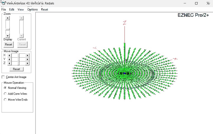
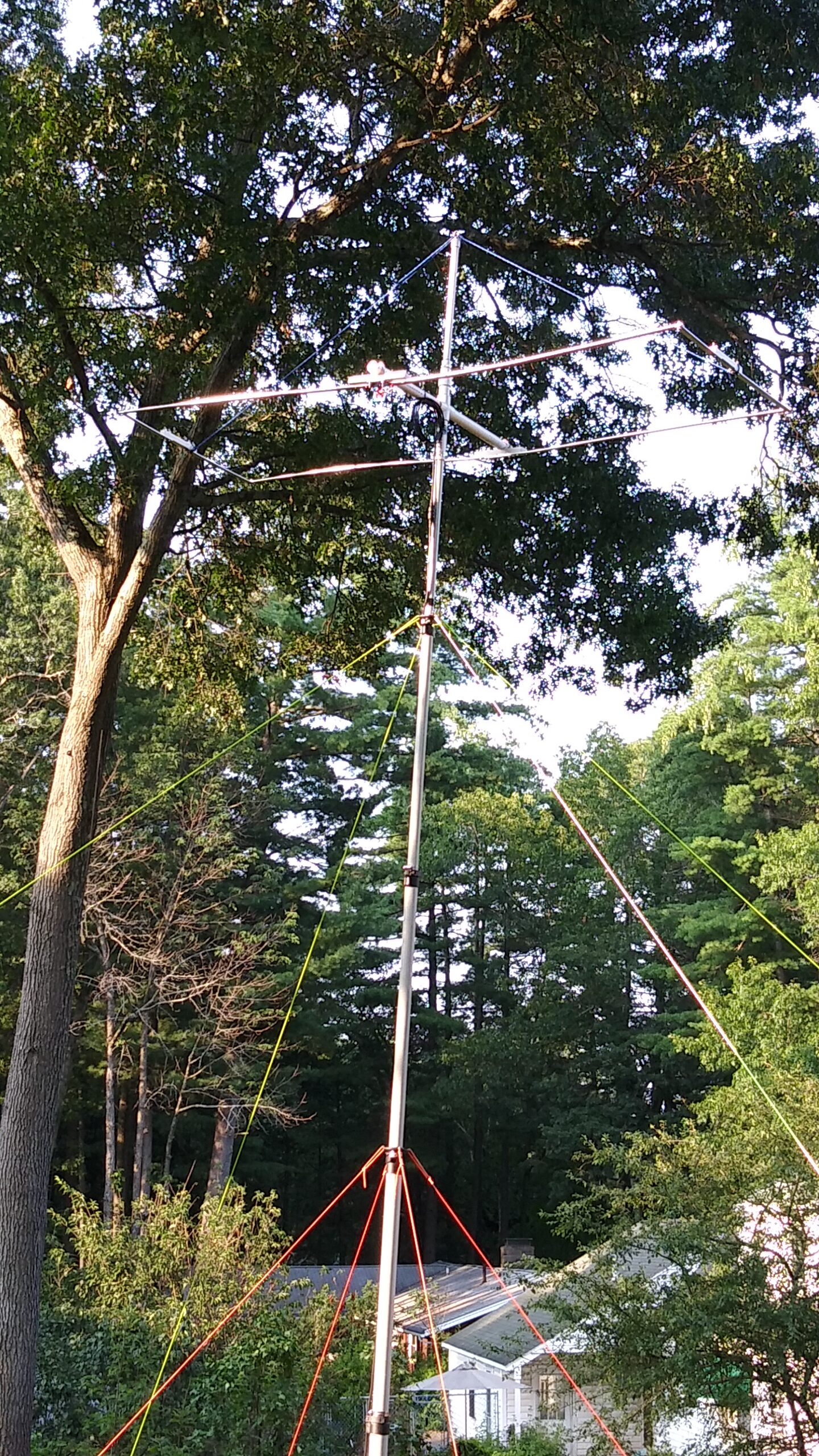
Jay KA1PQK set up his station for FT8 digital operation on 20 meters. His equipment consisted of a Yaesu FT-817ND radio operating at 5 watts, a MFJ-2286 Portable Vertical “Big Stick” 17 foot whip antenna with radials mounted on a Home Depot work light tripod, RG8x feedline, a Ryobi 18v Lithion Ion battery with a HomelyLife Voltage Reducer Automatic Buck Boost Converter (DC 8V-40V to 12V 3A 36W) to bring the battery voltage to that required by the radio. Jay used a Dell Rugged Tablet running WSJT-X for FT8 digital operation and also served as a logging tool. A RigExpert Stick Pro Antenna Analyzer was used to tune the antenna. Jay made 24 contacts, with the most distant being in Graham, Washington.

20m Station
POTA
20m Vertical Antenna

15 Meters

Jack WM0G used the opportunity to operate on the 15m band. His equipment consisted of an Elecraft KX2 at 5 watts with Elecraft MH03 handheld microphone, the internal KX2 tuner and KXBT2 battery, a MP1C Tunable Superantenna with precut radials, and 8 meters (25 feet) of RG8x feedline. For logging Jack used a Samsung Tablet running HamRS docked in a Jelly Comb Model# B046 keyboard (discontinued), with ARRL Logbook Mini as a paper backup.

Jack used the AEA model AA-30 antenna analyzer to tune the vertical antenna, and a Verizon Hotspot for internet access if needed.He also brought but didn’t use Heil BM-17 headphones and a Flashfish 200w solar generator. Jack operated using Upper Sideband SSB on 15 meters, making 5 contacts including four DX contacts to locations as varied as Norwich England, Haldensleben Germany, Dunajská Streda Slovakia, and Muscat, Oman, with the longest distance of 11,020 km (6,848 miles) with 5 watts and a portable vertical antenna!

WM0G POTA
15m Station
15m Vertical Antenna

10 Meters

Mike W1TKO used the day for experimentation and familiarization with some new equipment including a Xiegu X6100 radio at 5 watts and 12v sealed Lead Acid battery and 15 meters (50 feet) of LMR-240 co-ax feedline. One configuration used a Sirio SD27 rigid rotatable dipole tuned for 10 meters on a stout Manfrotto video tripod with the central tube removed to accept the mask of the antenna.  Another configuration used a home-brew End Fed Half Wave wire antenna with Pacific Antenna SOTA EFHW tuner on 20 meters, mounted just 3 meters (10 feet) off the ground between a tree limb and the pavilion roof.  Mike made just a few SSB contacts, logging with paper and pencil.  His most interesting contact was with another POTA operator in Kentucky with his 20 meter configuration.

10m and 20m Experimental Station
10 Rigid Dipole Antenna

Challenges Encountered

No portable operating event is without occasional challenges. In fact, this is one of the attractions of this type of amateur radio activity in that no two activations are alike. This section discusses some of the challenges encountered and how they are addressed in this or future activations.

Antenna tuning

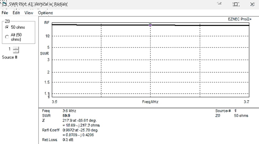
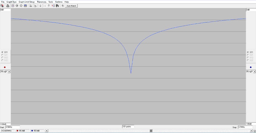
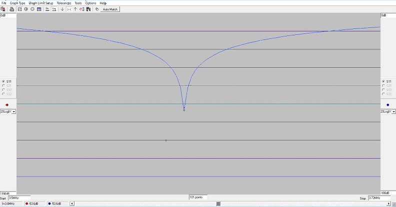
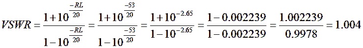
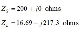
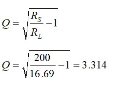
Antenna placement and tuning presented some challenges. An antenna analyzer is a critical piece of equipment for the rapid evaluation of the placement of the antenna and tuning of non-resonant antennas such as verticals.

One operator found his vertical antenna to be somewhat sensitive to small changes. To address this, he expanded the frequency range on the antenna analyzer to identify the resonant point of the antenna at its current position, and then adjusting the antenna coil to bring the frequency into the desired operating range.

Near Station Interference

Whenever several stations are operating in close proximity to each other, there is risk of adjacent frequency interference between them. Operators first listened on the intended band of operation and then chose an unused (at this location) band to maximize isolation between stations. One operator tuned across 40m and 20m, and finding them in use decided to operate on 15m with great success.

In addition, radios such as the Yaesu FT-817ND and the Elecrafts have pretty good internal filtering which may have helped reduce interference. One user of the Xiegu X6100, however, experienced significant interference. He felt the radio did not have very robust pre-selector filtering, such that the transmit of another POTA operator on a different band was overloading the receive signal.  Distorted transmissions were being picked up from these nearby radios, making it hard to hear distant stations.   

Forgotten Items

Operators learned pretty quickly that it is important to have a checklist to ensure that all required equipment is taken to the portable operating site. Also, some members utilize “go boxes” with essential equipment in preassigned places (such as cutouts in foam packing material) to allow quick verification that essential items are packed and ready to go.

WM0G POTA
A Place for Everything

Every participant also emphasized the importance of setting up and trying out equipment at or near home before venturing out on a portable operating excursion. Pack and carry out all the equipment intended to bring, and then when the inevitable missing component is found, the remedy is near at hand. This is also important to do if the equipment hasn’t been used in a while to ensure that everything is still operating as expected.

And of course, ensure batteries are fully changed prior to leaving for the activation site.

Equipment Failures

One participant was using gear that was new and this unfamiliarity resulted in several problems. The first symptom was inconsistent fluctuations in receive signal strength and SWR.  This was found to be caused by a loose connection within the antenna caused by making connections finger-tight where a tool should have been used, but this alone did not resolve everything.  A second issue was found to be an intermittent connection from a  cable’s PL259 crimped connector to its coax. Luckily, a spare length of finished coax was at hand, and replacing the cable resolved the issue.  Lessons learned include:

  • Try out new equipment close to home prior to travel to the operating site
  • Bring spares of commonly failing items, such as cables, fuses, etc.

Refinement

As is true for most amateur radio activities, there is always room for improvement. Participants are continually fine-tuning their portable operation equipment and methods.  Examples of observations made by participants include:

Packing

For this activation my gear was packed in a couple soft padded travel cases and put in my backpack.  I felt like I had too many cases to keep track of.  I’ve since moved my gear to Harbor Freight Apache cases.  One recent POTA activation I had everything in a medium case, but that took up a lot of room in my backpack (not much room left for layers or food).  Currently, I’ve shrunk my setup further to fit into a small Apache case.

Antennas

I’m also in the process of changing my antenna/tripod setup.

  • The Home Depot tripod is great, but really too big to carry around in a backpack.
  • I’m currently experimenting with a Grabil GRA-ULT01 MK3 lightweight portable tripod. I’m also looking at a smaller antenna – the Gabil GRA-7350TC.  I have done some comparisons on 20m between the MFJ 17 ft whip and the GRA-7350TC.  The MFJ, being 1/4 wave on 20m, has advantages.  The disadvantage is it still doesn’t fit in my backpack when collapsed…. might be time for a different backpack ;-). I still like the idea of a vertical – especially in areas that either don’t have trees, or where you really shouldn’t be throwing things up in trees.
  • Also, a vertical antenna generally has a stronger signal and gain at low takeoff angles than a wire antenna mounted too low (less than ½ wavelength) above the ground as a temporary wire antenna is likely to be. DX propagation benefits from a lower takeoff angle.

Extra Items

I plan to include an additional 25 feet of RG-8 coax with a barrel connector, allowing me the flexibility to extend my antenna further from my operating position if needed.

Simplicity

Adhere to the K.I.S.S. (Keep It Simple, Stupid) method when selecting your field operation equipment and antenna. I would rather spend more time on the air than troubleshooting rig, power, and antenna problems. Opt for setups that are quick to assemble and less prone to breakage.

In contrast, it’s possible to bring too much equipment on a POTA activation. One participant reported “Since I knew this POTA activation would be close to the car, I purposely went overboard and brought a little red wagon full for gear, tools, and parts.  It was a bit comical, but fun. For future outings, I want to streamline the gear I bring.  I’d also like to come up with a way to transport my portable setup where I could easily open up a carry case and things would be pretty much set to go, once I raise the antenna.”

Everything but the Kitchen Sink

Power Supply effect on Transmit Power

It is common to find that the power supply battery type and charge status has an effect on the maximum transmit power provided by the radio to the antenna. For example, both the Xiegu X6100 and the ICOM IC-705 have a max transmit power of 10w when operating from an external battery but only 5w when operating from the internal battery.

Jay KA1PQK was following up on a commonly held belief that the Yaesu FT-817 may reduce its output power to 2.5W when the input voltage falls below approximately 11V.  He originally used the buck/boost converter along with a 3S LiPo battery pack to maintain 12V as the pack’s voltage dropped.  From a little bit of internet browsing, he started to question whether or not the FT-817 actually drops its output voltage, or if it just flashes the power indicator as a warning that the voltage is getting low.

The easiest way to find out was to connect the FT-817 to a power meter, dummy load, and adjustable power supply, and test it.  He discovered that when the input voltage drops below about 11V, the power indicator starts flashing, but the output power REMAINS AT 5W!  He decreased the voltage all the way to 8V (the low limit of the FT-817), and output power remains at 5W all the way.

Experimentation

One participant reports, “I spoke with some visitors who were  interested in ham radio.  One fellow seemed to have interest in experimenting with and learning about home-brew antennas, very similar to myself.  As I am a relatively new ham, I could easily convey how much I’ve learned in the past two years thru NARS activities, by going to local hamfests, reading books & web sites, YouTube, and by hands-on experimenting.  I’ve learned ‘don’t be afraid to try.’ A lot of the time I get as much if not more enjoyment from trying to make something work as I do in operating it once (if ever) it’s fully functional.”

Future Portable Operating Events

NARS is hoping to schedule future events at a variety of locales, such as:

      • A park on an ocean beach
      • A mix of near-the-car POTA activations and one that’s more of a mild backpack/walk to the activation
      • A “Summits on the Air” (SOTA) event requiring a hike to the operating region near a mountain summit. SOTA often requires different equipment that is much lighter and easier to carry a distance in a backpack while hiking to the summit region, and easier to set up in a small space.

Conclusion

Portable and POTA activation is an attractive and rewarding amateur radio experience. No two sites are exactly the same, and the ham is continually challenged to address different antenna configurations, operating positions, and power sources.

If you are curious, come to an event and check it out. Even just the process of setting up, operating, and taking down gear will help refine your understanding of the radio operations, how to organize things, of what’s important and what’s not. Even if it’s not your gear, someone will likely appreciate you helping to set up or take down.  You can take a turn at operating, and overall it’ll make you a better and more capable operator.  It’s just a fun social activity to do it as a group, and spending time with friends in the great outdoors is a plus!

Matching to the Complex Load Impedance of a Shortened, Non-Resonant Antenna – Part II

Introduction

In Part I of this article[1], a method for matching the complex load impedance of shortened, non-resonant antennas using L-matching networks and resonators was described. First, we matched to the real part of the complex load impedance, ignoring the imaginary part – the reactance part – until the real part had been matched with an L-matching network. Then, we resonated out the imaginary, reactive part to cancel it, at least at a single design frequency. The technique of reactive absorption was also demonstrated to further simplify matching networks.

Some years ago, Phil Salas, AD5X, presented an interesting approach for matching non-resonant antennas in his QST articles[2][3]. In these, he describes a method for feeding a 43′ vertical antenna with a base-loading network. In his matching technique, he reverses the process used in Part I. First, he resonates out the imaginary part of the complex, capacitive load reactance with an antenna base-loading coil. Once that has been accomplished, he steps up the 50 ohm, real source impedance with a 4:1 voltage UNUN to a convenient, higher real impedance, 200 ohms. Finally, he locates a place on the base-loading coil that matches the stepped-up, 200 ohm, real source impedance. Procedures are provided for resonating away the reactance of the antenna load and for locating the position of the tap.

This article recaps the methods used in Part I and presents a new method for simplifying matching networks. Eventually, this leads us to AD5X’s solution for base-matching a 43′ non-resonant vertical antenna.

Discussion

Figure 1 illustrates AD5X’s method. A 4:1 UNUN transforms the 50 ohm transmitter impedance to 200 ohms. This follows because a 4:1UNUN has a turns ratio of 2:1 and the impedance transformation goes as the square of the turns ratio, N2 = 4. This results in a feed-point at a practical location on the base-loading coil and at a reasonable voltage, too, since the UNUN only increases the voltage by a factor of 2. For a 100 Watt transmitter, the voltage would be stepped up from 70.7 VRMS to 141.4 VRMS and for a 1500 Watt transmitter, the voltage would be stepped up from 274 VRMS to 548 VRMS. By practical location, it is meant that the feed-point is located at some distance from the end of the inductor so that adjustments may be made.

Figure 1. A 4:1 UNUN Feeds A Tapped Base-Loading Coil. The base-loading coil is tuned to resonate out the capacitive reactance of the shortened antenna. A point is found on the base-loading coil to inject the signal from the 4:1 UNUN and to achieve a match. Please click on the figure to enlarge.

Since the voltage increases by a factor of 2, the current must decrease by a factor of 2 according to physical law. The entire base-loading coil is tuned to be resonant with the antenna load capacitance (for our case 204.3pf) at the design frequency. This is the same technique that was used in Part I[4].

There is another way to think about the base-loading coil, however. It may be drawn as an L-network. The base-loading coil may be drawn as a parallel element and a series element, Figure 2. Instead of a conventional LC L-network, a less commonly used LL L-network is shown. This will be discussed in detail towards the end of this paper.

If operation on more than one band is desired, the base-loading inductor must be tuned to a new value to resonate with the antenna’s capacitive reactance in the new band. The tap position must also be moved. These changes may be implemented with movable jumpers[5], or they may be automated with relays[6].

Figure 2. A Simple LL Network. This LL network consists of two windings in series. It is easier to think about this device as a special case of an L-matching network. For multi-band operation, the inductor has to be re-resonated and the tap must be moved. This may be implemented with jumpers, or with relays. Please click on the figure to enlarge.

Commonly and Less Commonly Used L-Network Topologies

Part I described the four most common topologies for L-matching networks, shown in Figure 3[7]. These are not the only ones. There are four other simple L-networks, shown in Figure 4, that prove useful under some conditions, particularly if suitable inductors or capacitors are unavailable. For more information about these topologies, please refer to a book on the subject of Smith Charts such as Phillip Smith’s, Electronic Applications of the Smith Chart[8].

Figure 3. Four Commonly Used L-Matching Network Topologies. These topologies may be used to map and match the entire complex impedance plane. Please click on the figure to enlarge. Reproduced under CC BY-NC by permission of Michael Steer, North Carolina State University.

Figure 4. Four Less Commonly Used L-Matching Network Topologies. At a) and b), low-pass topologies. At c) and d), high-pass topologies. These topologies may be useful if suitable inductors or capacitors are unavailable. These topologies may be used to map limited portions of the complex impedance plane. The low-pass LL-version, RS > RL, is exploited towards the end of this paper. Please click on the figure to enlarge.

Modeling of a 43′ Non-Resonant Vertical Antenna in EZNEC

A 43′ non-resonant vertical antenna was modeled at 3.6 MHz in EZNEC[9] to find the unmatched feed-point impedance. For this case, 60 radial wires, 66′ (20.1m) in length (~1/4l) were used. The radials were placed 0.01m above the ground so that EZNEC could be used to model them. EZNEC instructions state that for wires placed low to the ground, the Real/High Accuracy ground type must be selected[10]. The soil conductivity was set to 6 mS/m, while the dielectric constant was set to 13.

The 43′ antenna model is shown in Figure 5. This model utilizes wire for the 43′ vertical. It could just as easily have been replaced with a piece of aluminum tubing. This would alter the antenna impedance. However, for this instructive exercise, it doesn’t matter.

Figure 5. The 43′ Non-resonant Vertical. The radials were modeled at ~1/4λ for 80m. Please click on the figure to enlarge.

EZNEC was run for a few points to obtain the unmatched impedance at 3.6 MHz. The result is shown in Figure 6. The impedance at the base of the vertical is ZL = 16.69 – j217.3 ohms. The VSWR is shown to be 59.9:1, and this will be calculated directly from the unmatched impedance. The capacitive reactance, -j217.3 ohms, equates to 203.4 pf at 3.6 MHz.

Figure 6. EZNEC Plot of the Unmatched 43′ Antenna with Radials. The frequency span is 3.5 to 3.7 MHz. The VSWR is calculated in a 50 ohm system. Please click on the figure to enlarge.

Calculation of the Unmatched VSWR from the Load Impedance

The unmatched VSWR is calculated from the simulated antenna load impedance ZL = 16.69 – j217.3 ohms. To determine the VSWR, the input voltage reflection coefficient is calculated for the unmatched antenna. The input voltage reflection coefficient is a measure of how much of the voltage wave incident at the unmatched antenna discontinuity is reflected back toward the RF source. As the voltage reflection coefficient approaches unity, more of the incident wave is reflected from the antenna discontinuity back toward the transmitter or signal source. The voltage reflection coefficient is calculated from

where

ZL is the complex load impedance of the antenna as simulated in EZNEC, or measured with a vector antenna analyzer, in units of ohms.

ZS is the complex impedance of the signal source, which could be the transmitter, or a vector antenna analyzer, in units of ohms.

For the time being, we ignore the 4:1 UNUN and provide a match between a 50 ohm source and the complex load impedance. The 200 ohm source impedance is introduced into the simulation for Example 3.

Given,

the value of the complex reflection coefficient is given by

Combining terms, where possible

Method I – Rectangular Form

Rationalize the denominator

The magnitude of the reflection coefficient is given by

The voltage standing wave ratio is defined by

The VSWR of the unmatched 43′ vertical is 59.97:1. This agrees with the EZNEC result.

Method II – Polar Form

and let

and let

Dividing, we obtain

Moving the angle from the denominator to the numerator changes the sign.

All we need is the magnitude, and it agrees with Method I

VSWR is defined by

For exercise , we may convert from polar form back to rectangular form

This value of the magnitude of the reflection coefficient agrees with the first result for a VSWR of 59.61:1.

Return Loss

The return loss is a measure of  the loss of signal power due to mismatch between the source impedance and the unmatched load impedance. By IEEE convention, the return loss is always expressed as a positive number in units of dB. The lower the return loss, the worse the mismatch is.

This agrees with the EZNEC result.

Mismatch Loss

If the antenna load impedance is mismatched to the source, the loss in units of dB will be

Forward Power

The forward power, expressed in units of percent, is

Reflected Power

The reflected power, expressed in units of percent, is

Impedance Matching Techniques Using L-Networks – 50 ohm Source Impedance

In Part I, techniques for matching with L-networks were introduced. In this section, L-networks will be used to match a 50 ohm source to the mismatched 43′ antenna. (We will visit the case of the 200 ohm source later.) Once the real part of the complex antenna load impedance has been matched, the reactive part will be canceled using the reactance adsorption technique for the first two examples. A new technique will be used for the third example.

It is known from Figure 3 that the  equations in the following sections apply for RS > RL.

Example 1 – Low-Pass Topology with Reactance Adsorption


We write down the equations that will match a real source impedance of 50 ohms to a real load impedance of 16.69 ohms. Thus, we set the reactive part of the load impedance to zero.

From Figure 3(b), we learn that for

the unloaded Q is calculated from

The L-network reactances and component values are calculated from

We are not done yet because we have ignored the reactive part of the antenna load impedance. This is, after setting the real part to zero

This impedance is equivalent to a capacitance of

We remember that to cancel a negative reactance, we need an equal but opposite positive reactance. So, we need a positive inductive reactance of

to cancel the negative capacitive reactance of the load impedance.

The required inductive reactance is calculated from

This resonating inductance may be combined with the series inductance in the matching network for a total inductance of

This matching network may be modeled in RFSim99 with the following results. Figure 7 shows the circuit model, while Figure 8 reports a return loss of 55 dB. Figure 7 does not combine the series inductors. They could be combined, but they have been modeled separately for clarity. The simulation result is the same.

Figure 7. Circuit Model of Low-Pass Topology. The low-pass network matches the 50 ohm source impedance to the antenna complex load. The resonating inductor has not been combined with the L-network inductor for clarity. See text. Please click on the figure to enlarge.

Figure 8. Plot of the Low-Pass Topology Return Loss. This simulation is for the 50 ohm source impedance to antenna complex load match. The return loss is better than 55 dB at 3.6 MHz. Please click on the figure to enlarge.

Calculate the VSWR

Let’s calculate the VSWR from the return loss. The return loss is defined as

If we solve for the magnitude of the reflection coefficient, we have

Finding the antilog of both sides, we obtain

VSWR is defined as

Substituting, we obtain

The VSWR is 1.004:1.

From the graph, the 2:1 VSWR bandwidth for this low-pass L-network is 180 kHz. This is based on a return loss of 9.54 dB for a 2:1 VSWR.

Now that the low-pass solution has been modeled, let’s perform a similar analysis for the high-pass solution.

Example 2 – High-Pass Topology without Reactance Adsorption

We write down the equations that will match a real source impedance of 50 ohms to a real load impedance of 16.69 ohms. Thus, we set the reactive part of the load impedance to zero.

From Figure 3(d), we learn that for

the unloaded Q is calculated from

The L-network reactances and component values are calculated from

As before, we are not finished because we have ignored the reactive part of the antenna load impedance. This is

after setting the real part of the load impedance to zero.

This impedance is equivalent to a capacitance of

We remember that to cancel a negative reactance, we need an equal but opposite positive reactance. So, we need a positive inductive reactance of

to cancel the negative capacitive reactance of the load impedance.

The required inductive reactance is calculated from

For the high-pass configuration of Figure 9, the resonating inductance may not be easily combined with the shunt inductor in the L-network. Later, we will show how the network may be simplified. Meanwhile, let’s model the topology that we have. The simulation results in the return loss plotted in Figure 10. The result is 53 dB at 3.6 MHz.

Figure 9. High-Pass L-Network Topology Return Loss. This topology matches a 50 ohm source impedance to the complex antenna load impedance. The resonating inductor is not easily combined with any other component in the L-network. See text. Please click on the figure to enlarge.

Figure 10. Plot of the High-Pass Topology. This simulation is for the 50 ohm source impedance to antenna complex load match. The return loss is better than 53 dB at 3.6 MHz. Please click on the figure to enlarge.

VSWR Calculation

Substituting, we have

The VSWR is 1.004:1.

The 2:1 VSWR bandwidth for this high-pass L-network is also 180 kHz. This is based on a return loss of 9.54 dB for a 2:1 VSWR. This bandwidth is consistent with the value reported for the low-pass L-network.

Example 3 – High-Pass to Low-Pass Transformation by Partial Reactance Absorption

This is an interesting solution to our impedance matching problem. It puts a number of the tools that we have learned to work and provides an interesting path for simplifying the results from Example 2.

Since our matching network begins with a 4:1 UNUN, that transforms 50 ohms to 200 ohms, and we can change the source impedance for our calculations from 50 ohms to 200 ohms.

We begin, as before, by writing down what we know.

We write down the equations that will match a real source impedance of 200 ohms to a real load impedance of 16.69 ohms. Thus, we set the reactive part of the load impedance to zero.

From Figure 3(d), we learn that for

the unloaded Q is calculated from

The L-network reactances and component values are calculated from

As before, we are not done yet because we have ignored the reactive part of the antenna load impedance. This is

after setting the real part of the load impedance to zero.

This impedance is equivalent to a capacitance of

We remember that to cancel a negative reactance, we need an equal but opposite positive reactance. So, we need a positive inductive reactance of

to cancel the negative capacitive reactance of the load impedance.

The required inductive reactance is calculated from

The circuit model for our matching network is shown in Figure 11. Note that, as was the case for Example 2, the resonating inductor is not readily combined with the other inductor in the matching network. We will fix this. The return loss, Figure 12, is better than 64 dB at 3.6 MHz.

Figure 11. High-Pass L-Network with Resonating Inductance Return Loss. The resonating inductance is not easily combined with the shunt inductor at the input. This will be remedied in the next step. Please click on the figure to enlarge

Figure 12. High-Pass L-Network Return Loss. The return loss at 3.6 MHz is better than 64 dB. Please click on the figure to enlarge.

The circuit model for the high-pass topology includes a resonating inductor that cannot be easily absorbed. Is there any transformation that can be applied to simplify the circuit? It turns out that there is. The key to this transformation is to write the series elements in the matching network in terms of their algebraic reactances in ohms.

Please recall that the 799.3pf capacitor had a complex reactance of -j55.31 ohms. The 9.607μH inductor had a complex reactance of +j217.3 ohms. If we add the two together, we obtain

The plus sign indicates that, at least at 3.6 MHz, we could replace the 799.3pf capacitor and the 9.607μH inductor with a single inductor possessing a reactance of +j162.0 ohms.

It is easy enough to work out the inductance value from

This is an interesting result. We have replaced an LC high-pass network with a resonating inductance with an LL low-pass network consisting of a shunt inductor at the input followed by a series inductor.

Now, it is time to go back to the model and see what happens. You might want to find the 2:1 bandwidth and calculate the VSWR from the return loss of this topology. Hint: The 2:1 bandwidth may be read off the plot between the -9.54 dB points. Hint: Use the formula for converting return loss to VSWR that appears in Example1 and Example 2.

Figure 13 shows the circuit model for the partially absorbed resonant inductive reactance. This topology employs one of the lesser-used LL L-matching networks. Networks of this type will match reduced portions of the complex plane, but the transformation topology works for us in this example.

Figure 13. Low-Pass LL Circuit Model with Partial Reactance Adsorption of the Resonating Inductor. This topology is one of the less-used L-matching networks. Networks of this type will match reduced portions of the complex plane, but the transformation topology works for us in this example. Please click on the figure to enlarge.

Figure 14 plots the simulation results for the low-pass LL L-network that is the result of transforming the high-pass network LC L-network. The ~200 kHz bandwidth appears to be somewhat of an improvement over the other topologies. The return loss is better than 59 dB.

We calculate the VSWR as we have done before

The VSWR is 1.0022:1. As an exercise, try calculating the mismatch loss, forward power and reflected power following steps outlined earlier to see the improvement.

Figure 14. Return Loss of the Low-Pass LL L-Network. The ~200 kHz bandwidth appears to be somewhat of an improvement over the other topologies. See text. The return loss is better than 59 dB for a VSWR of 1.0022:1. Please click on the figure to enlarge.

Please note that when entering the values into the RFSim99 circuit models, the values are rounded off by the app. These truncations result in precision errors that degrade the values for return loss. Inevitably, they lead to errors in reading off the 2:1 bandwidths. Nonetheless, the return loss values are excellent for all three of the matched cases.

There may be some cases for non-resonant antennas where an LL L-network will not work. We were fortunate that we could completely absorb the capacitive reactance of the original high-pass L-network. If the capacitive reactance is too large and the resonating inductive reactance is too small, we will be left with a capacitor in our matching network. This simply means that our load impedance is on a part of the complex plane onto which an LL L-network will not map. To learn more about this, please consider giving Phillip Smith’s book[11] a read. He presents a lot of good material on the subject of LL and CC low and high-pass networks including where they map.

Conclusions

This paper has provided a recap of material provided in Part I for a 43′ non-resonant vertical antenna. The method of partial reactive absorption has been introduced. For our mismatched antenna, we were able to convert from an LC high-pass matching solution to an LL low-pass matching solution. This results in a solution that does not require capacitors. This may not always be the case. It depends on where on the complex plane the antenna complex impedance is located. CC solutions are also possible, but not for our value of complex load impedance. As an exercise, try to figure out why. Hint: Smith Chart L-matching network mappings. The matching topologies introduced in Parts I and II are by no means comprehensive. More complex matching networks offer wider bandwidth, and these provide opportunities for future articles. Part III will discuss the topic of high voltages encountered in matching networks as well as high voltages resulting from highly reactive mismatches in non-resonant antennas.

References

[1] Blustine, Martin, K1FQL, Matching to the Complex Load Impedance of a Shortened, Non-Resonant Antenna – Part I, N1FD Article, July 6, 2023. https://www.n1fd.org/2023/07/06/matching-antenna-part-i/

[2] Salas, Phil, AD5X, 160 and 80 Meter Matching Network for Your 43 Foot Vertical – Part 1, QST, Dec. 2009, pp. 30 – 32.

[3] Salas, Phil, AD5X, 160 and 80 Meter Matching Network for Your 43 Foot Vertical – Part 1, QST, Jan. 2010. pp. 1 – 4. https://www.arrl.org/files/file/QST%2520Binaries/QS0110Salas.pdf

[4] Blustine, July 6, 2023, op. cit.

[5] Salas, Dec. 2009, op. cit.

[6] Salas, Jan. 2010, op. cit.

[7] Blustine, July 6, 2023, op. cit.

[8] Smith, Philip H., Electronic Applications of the Smith Chart, p. 115, McGraw-Hill 1969. https://www.scribd.com/doc/96997209/78897620-Electronic-Applications-of-the-Smith-Chart-SMITH-P-1969

[9] Lewallen, Roy, EZNEC, Antenna Software by W7EL. https://www.eznec.com/

[10] Lewallen, Roy, EZNEC Pro+ v. 7.0 Printable Manual. https://www.eznec.com/ez70manual.html

[11] Smith, Philip H., op.cit.

Truss added to DIY 6m Moxon Antenna

6m Moxon with vertical extension and a rope to each end
6m Moxon with truss and safety-color guy lines

Back on July 17, 2022, I made a post here about building a DIY Moxon antenna for 6m based on plans in the ARRL book Magic Band Antennas for Ham Radio by Bruce Walker N3JO.  It was made of flat aluminum bars instead of round tubing.  The problem with it was that the ends drooped significantly, which reduced the directionality.

I expected this, so I used a cross instead of a ‘T’ in the middle of the boom.  That let me add a vertical extension of PVC pipe in the middle of the boom.   I drilled a hole in the top of a PVC cap, mounted a (stainless steel) eye-bolt in the hole, and put it on top of the extension.  (With the mast lying on the ground, of course.)  Then I was able to tie paracord from the eye-bolt to each end of the antenna as shown in this picture.  I am more concerned about accidents with the lawn mover than stealth in my back yard, so you can see that I used bright safety orange and safety yellow-green paracord for the guy lines.  (In fact, my neighbor, also an engineer, commented that this was a good idea, to prevent tripping.)

I used the “Orange Screw” product mentioned here by others to anchor the guy lines to the ground.  I also used hose clamps, in addition to the mast’s own clamps, to keep the mast from telescoping inward.

It’s important to remember that the only two knots to use with antennas are:

  1. the taut-line hitch and
  2. the bowline knot.

(To help with pronouncing the later, try to remember that it was named for the front end of a boat, where sailors use it.)  These knots were covered in the Tech Night presentations about Field Day.

Aron, W1AKI

Radio Amateurs Developing Skills Worldwide