In Part I of this three-part series, differential and common modes on RF transmission lines were defined and discussed.
In Part II of this article, the work of Gustav Guanella was chronicled, followed by Joe Reisert’s improvements to Guanella’s original design. The construction of a common mode choke was presented that included data for the coax used. Finally, some analyses were performed that predicted the performance of two common mode chokes. Graphical results were reported.
In this final Part III, the results of measurements performed on two common mode chokes are presented: one for 2 x FT240-31 stacked ferrite cores and another for 2 x FT240-43 stacked ferrite cores. Due to its higher initial permeability, it was expected that low-frequency choking performance for the 2 x FT240-31 material would be superior to that of the 2 x FT240-43 material. We found that this was not the case for the single sample of 2 x FT240-31.
Discussion
Two coaxial line chokes were constructed to suppress common mode currents on transmission lines. Common mode currents are apt to find their way back to the operating location on the coax shield. Common mode currents can create performance problems in the form of added receiver noise and operator problems in the form of RF bites. The choking impedance should be located at a voltage node in the feedline where the wave impedance of the standing wave is low.
The coaxial line chokes were constructed on stacked cores of FT240-31 and FT240-43 material, as the literature recommends both for EMI suppression. Eleven turns of RG-400/U coax were wound on each of the stacked cores with the Joe Reisert, W1JR, crossover winding located in the center. Each choke was housed in a connectorized Bud Industries PN-1323 box. The common mode rejection for each choke was measured with a spectrum analyzer over a 1.8 to 29.7 MHz bandwidth. The spectrum analyzer tracking generator output was split into two in-phase signals that fed the choke coax center conductor and the choke coax braid in true common mode. The resistive divider formed with two 25.5-ohm resistors (made with 51-ohm resistors in parallel) is shown in Figure 1. The divider was fed in the center by the tracking generator and the ends of the 25.5-ohm resistors fed the center conductor of the coaxial connector and the connector shell. There was a similar arrangement at the output so that the spectrum analyzer could measure the resulting common mode rejection. The conduction path of the test cable shield was carried from input to output on #16 AWG as shown. Figure 2 shows the device under test. Some undesired responses were due to some nearby equipment, coax and line cords. The distance between the test coax shields also presents some challenges, and an interconnection bridge is shown that consists of a rather long piece of #16 AWG wire. After moving some cables, line cords, and equipment around, some useful data was collected. Figure 1 – Feeding the Common Mode Choke in Common Mode. A resistive power divider was constructed that consisted of paralleled 51-ohm resistors to make two 25.5-ohm resistors. The center conductor of the choke coax and the choke coax shield were fed with in-phase signals from the spectrum analyzer tracking generator. Figure 2 – Recombining the Common Mode Signals. Similarly, a resistive power combiner was constructed at the choke output that consisted of paralleled 51-ohm resistors to make two 25.5-ohm resistors. The in-phase signals from the center conductor of the choke coax and the choke coax shield are recombined and fed to the spectrum analyzer input. The shield from the input coax and output coax is bridged with a piece of #16 AWG copper wire as shown.
The reference level of the spectrum analyzer was set for -10 dBm and all measurements were made relative to that level. The first screenshot is for 11 turns of RG-400/U wound on 2 x FT240-31, while the second screenshot is for 11 turns of RG-400/U wound on 2 x FT240-43 material. Since the toroids are wrapped with the same number of turns of RG-400/U, the #31 material, possessing higher initial permeability, is expected to exhibit a higher choking impedance at 1.8 MHz than the 43 material. This does not appear to be the case for this batch of #31 ferrite. The provenance of the #31 material is good. In any event, there is greater than 20 dB of common mode rejection for both ferrite types from 1.8 to 29.7 MHz. While the response appears to favor low frequencies for #31, the overall suppression is better for this batch of #43 material. No loss corrections have been made for the resistive power divider or resistive power combiner. Figure -. Suppression of a 2 x FT240-31 Line Choke. The ferrite material favors the lower bands but the overall suppression is inferior when compared to that of the 2 x FT240-43 line choke. Deconstruction of the choke may disclose some defects in materials or construction. Only a single choke of this type was constructed. Figure 4 – Suppression of a 2 x FT240-43 Line Choke. The ferrite material favors the higher bands but the overall suppression is superior when compared to that of the 2 x FT240-31 line choke. Fortuitously, several chokes of this type were constructed.
Conclusions
A single choke was constructed with FT240-31 material while several were constructed with FT240-43 material because most of our operation is above 7 MHz. While the shape of the response appears to favor low frequencies for #31, the overall suppression is far greater for this batch of #43 material. These measurements will be repeated when another batch of FT240-31 material is obtained. Furthermore, it is possible that the deconstruction of the FT240-31 choke may disclose some construction or material defect.
Lately, there has been quite a bit of nice DX out there on the HF bands. If you are like me, you have a modest station to work from (100 watts and a wire antenna or two), but still like to chase DX. Often, you’ll hear lots of other “1 landers” working the DX station, but you can’t ever seem to break the pileup. Well, I have a few suggestions I’ve gathered over my 30 years of DX’ing and contesting that I’d like to share, which might help you get a few new ones.
One universal “truth” I have found though, above all others, is that working DX on CW is infinitely easier than working DX on SSB. If you have not yet jumped in to learn CW, I highly advise it if you want to be a successful DX’er and work the rare ones from a modest station. FT-8 / FT-4 is a bit of a different animal, and not all of what I will share is applicable to those digital modes, so I am going to focus on CW and SSB (although I work a lot of FT-8 and FT-4).
Without further ado…
#1: Listen, Listen, Listen
Did I mention you should listen? This is the first step in the process to catch that needed country. Almost all of my other recommendations stem from this… don’t be the alligator on the calling frequency… ever. A good DX’er listens far more than they transmit.
#2: Use a DX Cluster
I recommend using a DX Cluster for finding the DX. It is much easier to find the choice DX if you have others looking for it too! If you’re not familiar with a DX Cluster, there is a good primer here. If you are but aren’t sure which to connect to, I recommend W1DX (dxc.dxusa.net:7300), unless you use Ham Radio Deluxe, in which case I suggest WA9PIE-2 (hrd.wa9pie.net:8000). They both run the DXSpider cluster software. When you use a “cluster”, you might want to set a few filters to get rid of the spots (the reports of DX activity) you don’t really want to see. Here is a couple that work on DXSpider to get you started.
From the cluster, console enter the following to only see DX spots originating from US and Canadian stations…
Disconnect from the cluster, and then reconnect. At this point you should only see DX spots from US and VE stations
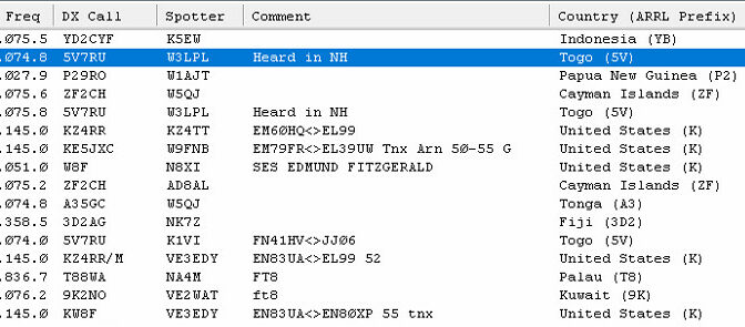
Typical DX Cluster screen
#3: Find and Hear the DX Station’s Calling Frequency
Once you identify the DX you want to chase, go find them on the air. Sometimes, that is easier said than done. Here’s where a set of good headphones and your radio’s RX IF filters will really come in handy.
Wearing headphones is important because they filter out all that background noise. If they are good headphones, they can also enhance the audio you are listening to and reduce fatigue.
As for your radio’s RX IF filters, this is where you may need to “RTFM”. Most modern HF radios will have some form of IF filter or DSP to shape the received audio. On Yaesu radios, they are “Width”, “Shift”, “Contour”, and “APF”. I won’t go into detail about their use here as all radios will be a bit different. I will say, however, that learning to use them is a critical part of effectively hearing the DX station. Ultimately, you can’t work ’em if you can’t hear ’em. Do not start calling the DX until you can reliably hear them.
#4: Find Where the DX is Listening
DX stations will listen in one of two ways… simplex (same TX and RX frequencies) or split (different TX and RX frequencies). Sometimes, the spot on the cluster will tell you where to start. However, many times the spots are not entirely right.
Simplex
If DX is working simplex, you are all set as to finding their RX frequency, but trust me… working rare DX simplex can be very difficult and painful. Always pray for split ;).
Split
If they are working split, finding the RX frequency can be a little challenging. Remember, working split means the DX station is transmitting on one frequency and listening somewhere else. Notice I didn’t say “on another frequency” – this is important to recognize. Many times, if the DX is listening on only one frequency, you can determine this from the DXCluster spot (i.e. “up 5”, which means that they are listening up 5 kHz from their TX frequency (such as TX: 28.507 / RX 28.512). However, often the DX is listening in a range of frequencies (i.e. “up 5-10”), which means they are listening somewhere between 5 and 10 kHz from their TX frequency (such as TX: 28.507 / RX 28.512 to 28.517). Now comes the fun part.
If the DX is listening split, it’s your job, as a skilled DX’er, to figure out their strategy and exploit it. Remember, even if the DX says “listening up 5”, they may not be listening up 5. They may in fact be listening up 7.2 or 9.3 or 3 kHz. Your job is to figure that out. Recently, I worked a DX station on CW that would sign “UP 1”. He was actually listening up 1.3 kHz. Had I simply called him up 1 kHz, I would not have worked him.
Patterns
To figure out their pattern and have a strategy to exploit it, you have some work to do, and likely some frustration in your future. It’s all worth it, though, if you bag an ATNO (All Time New One). Here are some steps to follow to find the DX stations listening frequency if they are working split.
Use the “split” function of your radio (you do know how to use “SPLIT” on your HF rig, right?). Set the “A” VFO to your RX frequency and the “B” VFO to a TX frequency where you think the DX is listening.
When the DX answers a station (i.e. “W1ABC UR 599”), flip the VFO’s so you are listening on the “B” VFO (or use your dual receive). Now find the station that the DX answered as they give their report. This can be tough, but is essential, especially if the DX is listening across a range of frequencies. Finding the station answering the DX gives you an idea of where the DX is actually listening. Do this until you can find/hear a station that the DX answered.
You can now do one of two things… flip the VFOs back and start calling the DX on the frequency you found that the other station was using, or you can keep listening to find if there is a pattern (like is the DX creeping up the band, down the band, moving 500 Hz at a time, staying put, etc). Once you can figure this out, your chances of working the DX greatly improve. When you’ve got their pattern (most DX stations will have one), flip your VFOs and work ’em. Repeating the process as needed.
[Side Note – Being DX
An important side note on being a DX station that may help you be better able to work them… a good DX operator will (in my opinion):
Work split. Simplex is fine if the DX is an everyday DX station like Poland or England. However, if they are even semi-rare, and expect pileups, they should work split. Simplex makes working rare DX very hard. The DX’ers have to separate the DX from the calling stations, which can be nearly impossible if the stations in the pileup call over top of the DX (which they do most of the time). IMO, simplex is bad.
Manage the pileup. Managing a pileup is hard and is a learned skill. To manage a pileup, the DX operator needs a strategy. It could be nearly anything, but having a strategy allows the DX to work more stations more efficiently and with less fatigue, and makes it easier for skilled DX’ers to work them.
]
#5: Use Your Rig’s “Monitor” Feature
If you’re working SSB, use your rig’s “Monitor” feature to listen to your transmitted audio. Do this to make sure it is not overdriven and sounds good. If you can adjust your TX audio as many new rigs can, do a little work to determine the best TX audio configuration for your voice and equipment. For many voices, there are differences in DX versus Rag Chew TX audio settings. For this, Google is your friend. (I recommend using “Monitor” for CW as well… lets you hear the quality of your transmitted tone too).
#6: Call High / Low
If you’re working CW and having a hard time working the DX on what you know is the correct frequency, try calling 100 Hz up or down from there. Sometimes that will serve to separate your signal from the others enough to work them. Due to the width of SSB signals, this rarely works on SSB, but can. Experiment.
#7: Watch Your Keying Speed
Also for CW… ideally you will match the DX’s keying speed. If they are calling at 35 WPM, call them at 35 WPM. You can go slower, but do not exceed their speed, as they may be at the top of their capability. If you send back at 45 WPM, you might never work ’em. Sometimes, however, if the pileup is full of speed demons on the key, sending a little more slowly will allow your signal to stand out. Again… experiment.
#8: Be Patient
I mean this in more than one way… it may take a while to work that ATNO, but patience on the mic or key can also pay off. While you are listening, notice if the DX is responding to stations quickly after calling “QRZ” or if there is some “dead” space in there. If there is a delay between “QRZ” and the DX responding, that may indicate that the pileup is all calling at the same time, immediately following the “QRZ”, making it impossible for the DX to discriminate calls; and the DX is waiting for a “laggard” to call them after the main pileup has finished. Be that laggard! Wait 3,4, or 5 seconds and then make your call. You might be the lone voice the DX hears!
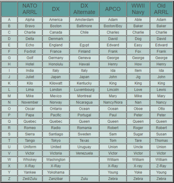
#9: Use Proper Phonetics
Many stations like to use their own phonetics “Wally One Finger Licking Good” may sound funny, but when the conditions are marginal, there’s a huge pileup, and the DX’s first language is not English; you might as well hang up the mic. Use proper, recognized phonetics so the DX can understand your call. K0NR has a great document on proper phonetics.
#10: Use the DX Station’s First Language
I have found that using the DX station’s first language can give a 10 dB gain to your signal LOL. So, if you speak German, French, Spanish, or any other language and you find a DX station that speaks that, use it to your advantage!
To “Tail End” or Not?
While not a recommendation (hence no number), I wanted to address “tail ending”. This can be a controversial tactic, but it can also be very effective if done correctly.
Tail-ending is when you throw your callsign out at the very end of someone else’s report to the DX (for example you say “November One Xray Yankee Zulu” as soon as “K5AAA” finishes his report. It goes something like this (K5AAA says: “P5DX, UR 599 in Texas” and you immediately say “November One Xray Yankee Zulu”).
Depending on how quickly the DX responds to K5AAA and how they feel about tail-ending, you might be able to work them by doing this. Some DX do not like that practice and will not respond to “tail-enders”. Best to either see if others are successful with this or don’t do it. I personally do not like this tactic, but it can be effective (especially in contests).
Putting it Into Practice
Before you start using these tips… look back at tip #1. Your ears are your best tool to successfully work DX. Of course, there are times that you simply won’t work a DX station no matter what you do. I had that issue on the very morning I wrote this… 30 minutes of using every trick I know, and I still didn’t work them before their signal faded.
So there you have it… my top 10 list of strategies to be a successful DX’er. As always, your mileage may vary, and others may have a completely different list. Every little trick helps in my opinion. Whatever strategies you choose to employ, just get out there and have fun.
In case you are curious, I have been on both sides of the pileups, working as the DX from a number of locations with very large pileups, as well as working from my home as the DX’er. At home, I rarely run more than 100 watts and have never had more than wire antennas or a vertical… unfortunately no beams have ever graced my yard. Yet, I’ve been successful in working DXCC in a weekend during contests, and have worked DXCC on 5 bands. I finally have a good 160M antenna up, so maybe I’ll increase my country count there too in 2023!
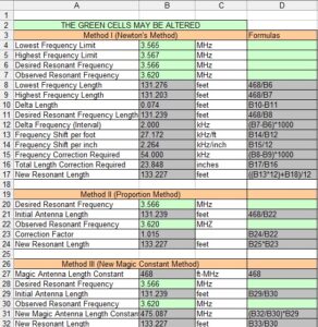
Whether it is for a half-wave dipole or an end-fed half-wave antenna, sooner or later we will have to prune one of these antennas to the correct length. Most of us are accustomed to trial-end error when it comes to tuning a dipole, but there are better ways to do it [1]. This paper describes three methods for your consideration. All of the formulas for the techniques shown may be entered into an Excel spreadsheet. If you do not have Excel on your computer and you have access to Google, you can use Google Sheets [2]. If you have Windows on your computer and have registered, then you can log into your Windows account and use Excel for free at office.com [3]. All three computation methods described may be entered onto a single spreadsheet, as in Figure 1, or entered onto separate tabs. All three techniques will produce the same answers. Most everyone owns a smartphone, so you can bring your spreadsheet app to the yard with you.
Directions for Loading the Spreadsheet
Figure 1 lists the spreadsheet formulas in Column D. Type these formulas over into Column B. Begin typing in Row 8, Column B. You must type an equal sign in front of every formula for the sheet to work. Once the formulas have been entered, enter the variables in the green cells in Column B. It is a good idea to lock the gray cells to protect the formulas from being over-typed. Then, protect the entire sheet so that the only cells open for data entry will be the green cells in Column B. If you click on Figure 1, it will open into a new window for easier viewing.
Figure 1. Sample Spreadsheet. Any one of the three methods or all three may be entered onto a single spreadsheet, or onto multiple spreadsheet tabs. A spreadsheet app on your smartphone is an easy way to carry the calculator to the field.
Descriptions of the Methods Used
Method I – Newton’s Method
The first method is one invented by Isaac Newton, but not for antennas. Newton was working with what we now call differential calculus in the late 17th century, which helps to put his genius into perspective. These days, we learn this technique in the first few weeks of calculus in high school. If we use the familiar formula to calculate the length of the dipole at a frequency just above and just below the desired frequency we can get a frequency differential.
If we subtract the two lengths, we get a length differential. By dividing the frequency differential by the length differential, we arrive at the number of kHz the resonant frequency moves per unit of length pruned. If we choose a very narrow frequency interval around our desired frequency, this technique becomes very precise. It’s a kind of sensitivity analysis. We move something a little bit and something else changes a little bit. That’s a hint as to what calculus is all about.
Method II – Proportional Method
The second method, which we call the proportion method, uses the familiar dipole length formula to arrive at the dipole length at a design frequency. In the field, we measure the frequency at which the antenna actually resonates. If we divide the observed frequency by the desired frequency, we arrive at a correction factor by which we multiply the old length to get the new length.
This is the most commonly used method for pruning an antenna.
Method III – New Magic Constant Method
The third and last method is called the “magic constant” method. We all remember that we divide 468 by the frequency in MHz to arrive at the dipole length in feet. The number 468 is what we call the “magic constant.” Suppose we calculate the length of a dipole using the magic constant. In the field, we observe that the dipole resonates at a different frequency. If we divide the observed frequency by the desired frequency, we arrive at a correction factor that can be multiplied by the old magic constant to get a new magic constant.
Then, we use this new magic constant to calculate a new antenna length.
Of the three methods, only the first method is a bit arcane because it uses differential analysis. The latter two are equivalent because they use proportions.
We use cookies to ensure that we give you the best experience on our website. If you continue to use this site we will assume that you are happy with it.

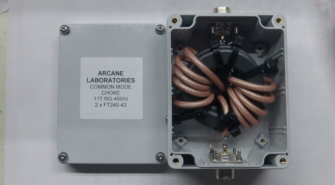
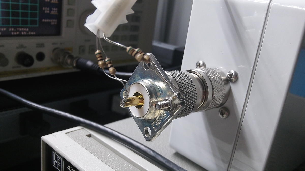 Figure 1 – Feeding the Common Mode Choke in Common Mode. A resistive power divider was constructed that consisted of paralleled 51-ohm resistors to make two 25.5-ohm resistors. The center conductor of the choke coax and the choke coax shield were fed with in-phase signals from the spectrum analyzer tracking generator.
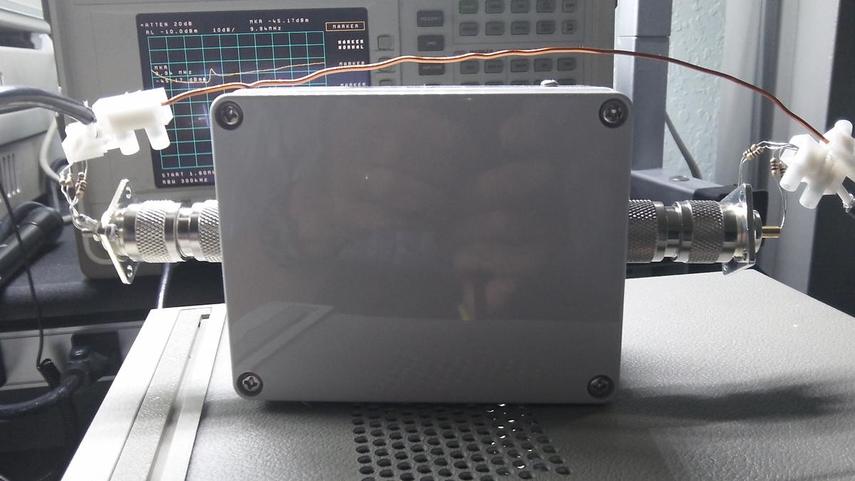 Figure 2 – Recombining the Common Mode Signals. Similarly, a resistive power combiner was constructed at the choke output that consisted of paralleled 51-ohm resistors to make two 25.5-ohm resistors. The in-phase signals from the center conductor of the choke coax and the choke coax shield are recombined and fed to the spectrum analyzer input. The shield from the input coax and output coax is bridged with a piece of #16 AWG copper wire as shown.
 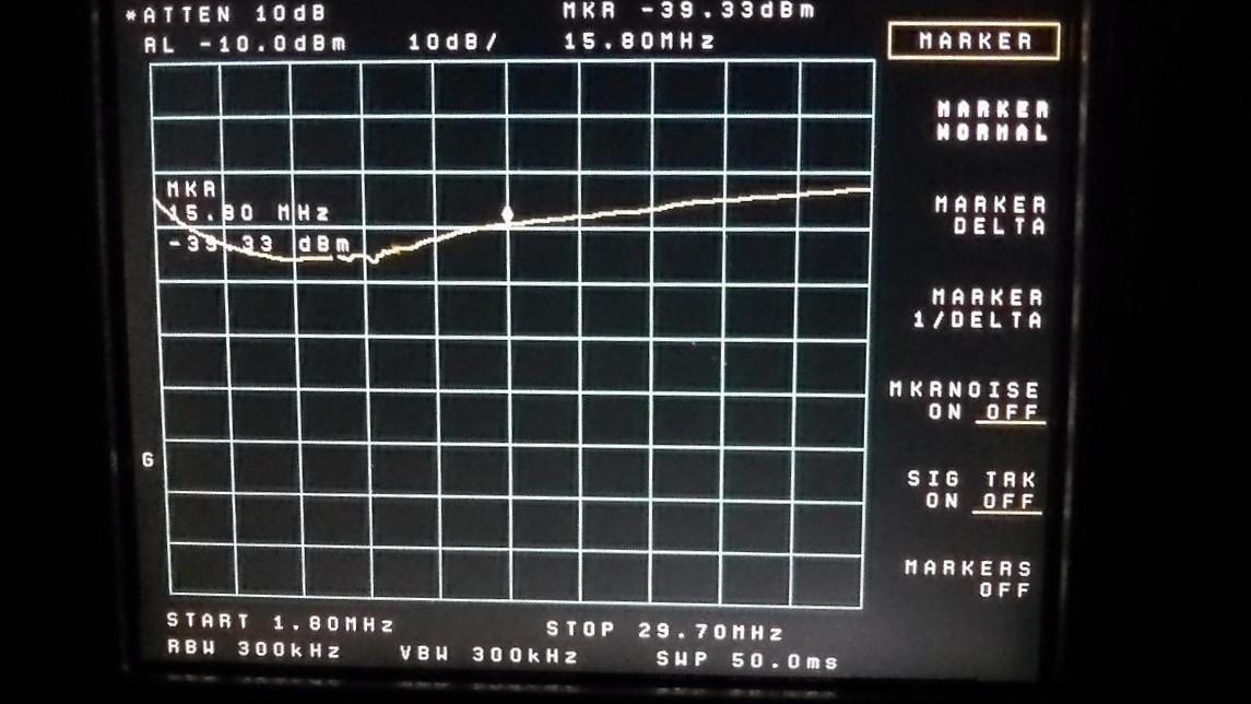 Figure -. Suppression of a 2 x FT240-31 Line Choke. The ferrite material favors the lower bands but the overall suppression is inferior when compared to that of the 2 x FT240-43 line choke. Deconstruction of the choke may disclose some defects in materials or construction. Only a single choke of this type was constructed.
 Figure 4 – Suppression of a 2 x FT240-43 Line Choke. The ferrite material favors the higher bands but the overall suppression is superior when compared to that of the 2 x FT240-31 line choke. Fortuitously, several chokes of this type were constructed.