Matching to the Complex Load Impedance of a Shortened, Non-Resonant Antenna – Part I
Introduction
A common impedance matching problem is that of matching a 50 ohm transmitter to a shortened non-resonant antenna. Examples of non-resonant antennas are the 23-foot (7.01m), and the 43-foot (13.1m) backyard vertical antennas. These antennas have something in common. They exhibit high capacitive reactance.
It is hoped that this multi-part article will provide the reader with the tools necessary to contend with this common antenna matching problem.
Part II of this article will discuss impedance matching to a 43-foot backyard vertical antenna using a 1:1 UNUN and an autotransformer[1].
The high voltages developed in these matching networks will be the subject of Part III of this article[2].
Example 1: 23-Foot Backyard Non-Resonant Vertical Antenna
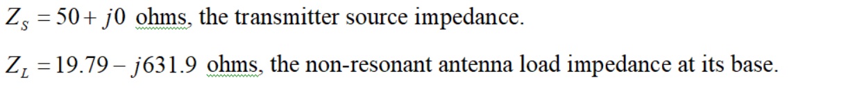
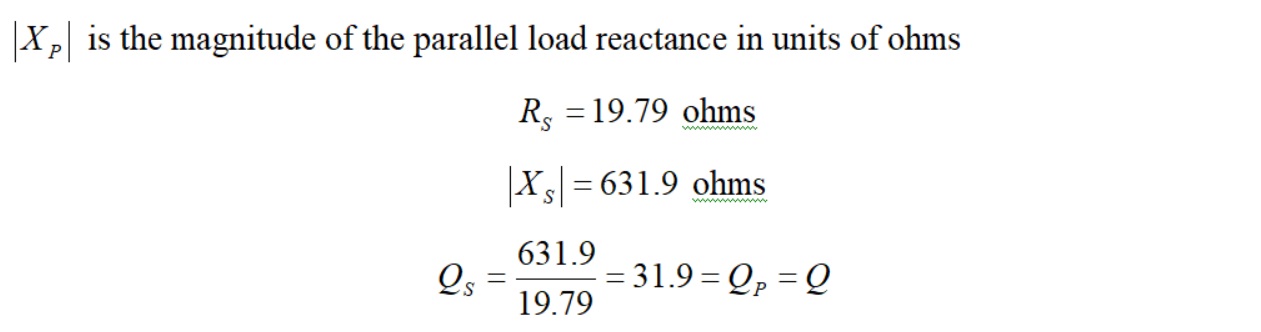
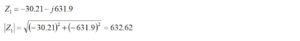
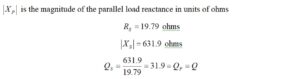
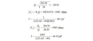
A 23-foot backyard vertical with numerous radials exhibits an impedance of 19.79 – j631.9 ohms at 3.6 MHz at its base.
For this exercise, we don’t care about the number of radials, conductor losses, ground losses, and reflected power that all figure into efficiency. All we care about is matching to this complex impedance.
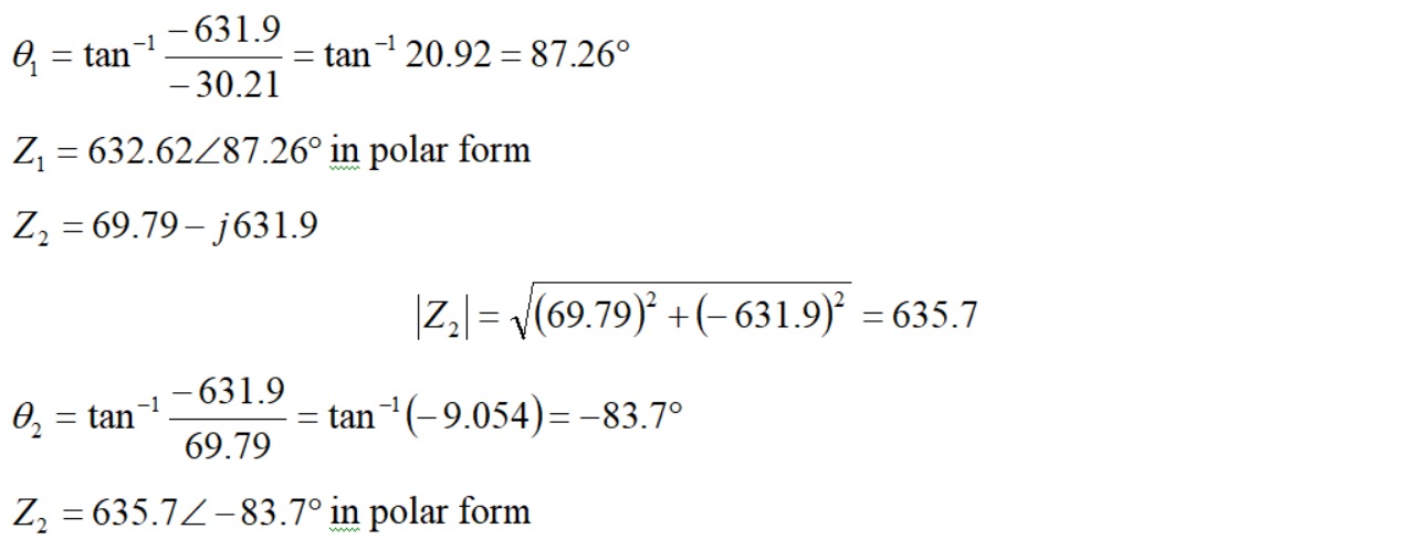
Unmatched VSWR
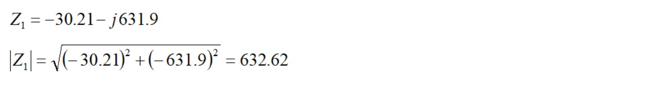
Let’s calculate the unmatched VSWR at the base of our 23-foot backyard vertical before we apply matching techniques. The load impedance that must be matched is assumed to be

The source impedance of the transmitter is given by

To calculate VSWR, we need to relate these two complex quantities to the magnitude of the reflection coefficient,

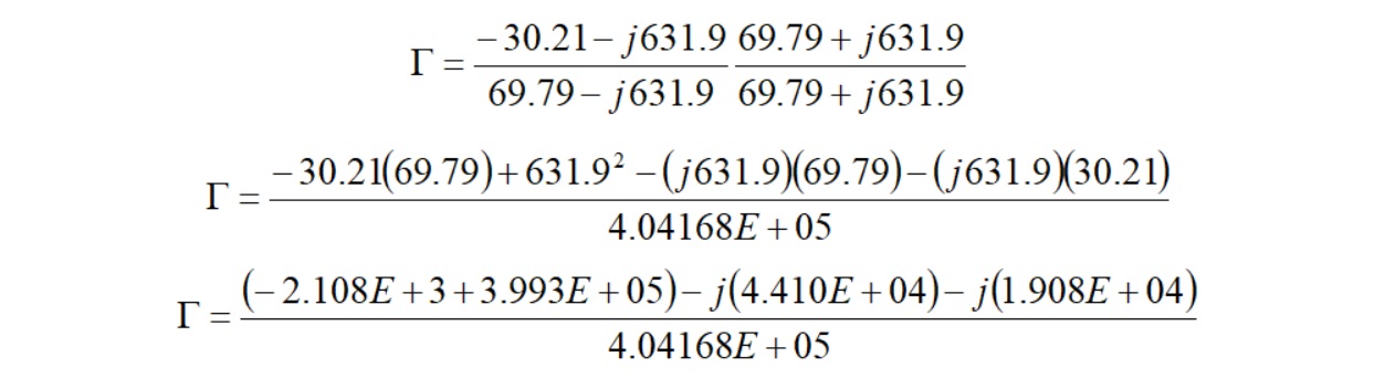
Those of us who own nanoVNAs have become used to the term S11, which is the input voltage reflection coefficient. By definition

This is a complex number that has to be rationalized before its magnitude can be found.

We should begin by combining terms where possible.

VSWR: Method I – Rectangular Form
Rationalize the denominator.
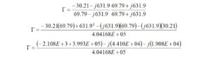
Like terms are combined to find the reflection coefficient.

The magnitude of the reflection coefficient is obtained from

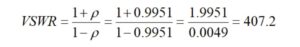
Finally, the VSWR is computed from

The VSWR is 406:1 due to the high value of capacitive reactance.
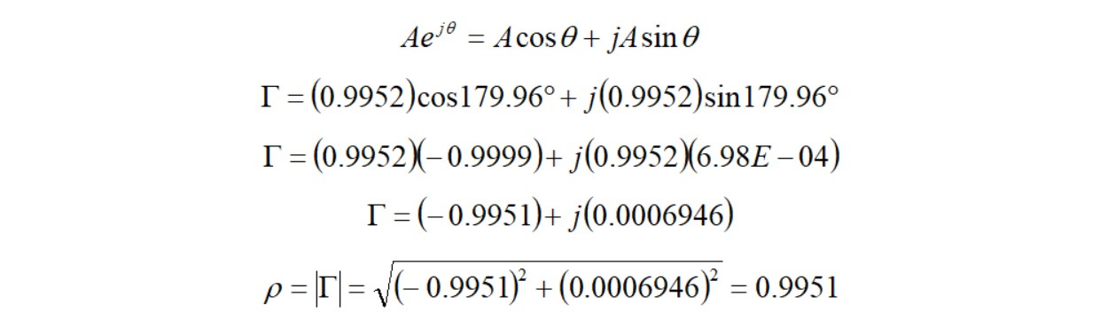
VSWR: Method II – Polar Form
As before, and after combining terms, we begin with

and let
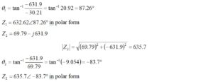
By dividing Z1 by Z2, we obtain

Notice that when the angle is moved from the denominator to the numerator, the sign changes.

We may stop here since we already have what we need

or, for the exercise, we may convert back to rectangular form using the Euler identity and arrive back at the same place.
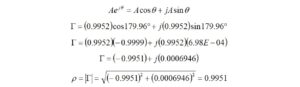
Rectangular and polar forms lead to the same result.
The high VSWR is due to the high value of capacitive reactance of the unmatched load impedance.
Matching Techniques
When faced with problems like these, it is often easier to break the problems down into more manageable steps.
How to match the real part of the load impedance was the subject of an earlier paper[3] but let’s review the procedure for this case.
We begin by inspecting the impedance to see what we can learn about it. The real part is 19.79 ohms. This resistance, RL, is smaller than the real 50 ohm transmitter impedance, RS. If we were to use a simple LC matching network, an L-network, we can see from Figure 1 that there are four possible topologies: two low-pass topologies and two high-pass topologies[4]. Notice that the low-pass topology is capable of conducting DC from input to output. This is not possible with the high-pass topology that blocks DC with a series capacitor. We begin by picking the low-pass topology in Figure 1(b) for which RS > RL.
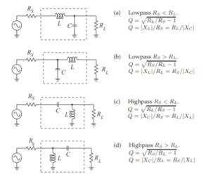
Figure 1. L-Matching Network Topologies. Source and load impedances are real. Reproduced under CC BY-NC by permission from Michael Steer, North Carolina State University.
It is instructive to work through low-pass and high-pass topologies to illustrate how these problems are solved. It is important to note that all of these solutions result in an impedance match for a narrow band of frequencies. If multi-band operation is required, the use of multiple matching networks or the use of an antenna tuner (preferably a remote one) will be necessary.
Other matching techniques are possible, such as center loading and top loading but we will limit the discussions in Part I, Part II, and Part III to base loading.
Example 1: Low-Pass Topology
We begin by writing down what we know,
Step 1
We set the imaginary part of the load impedance, ZL, to zero for Step 1 of the solution. We will revisit the reactive part in Step 2 of the solution.
Thus,

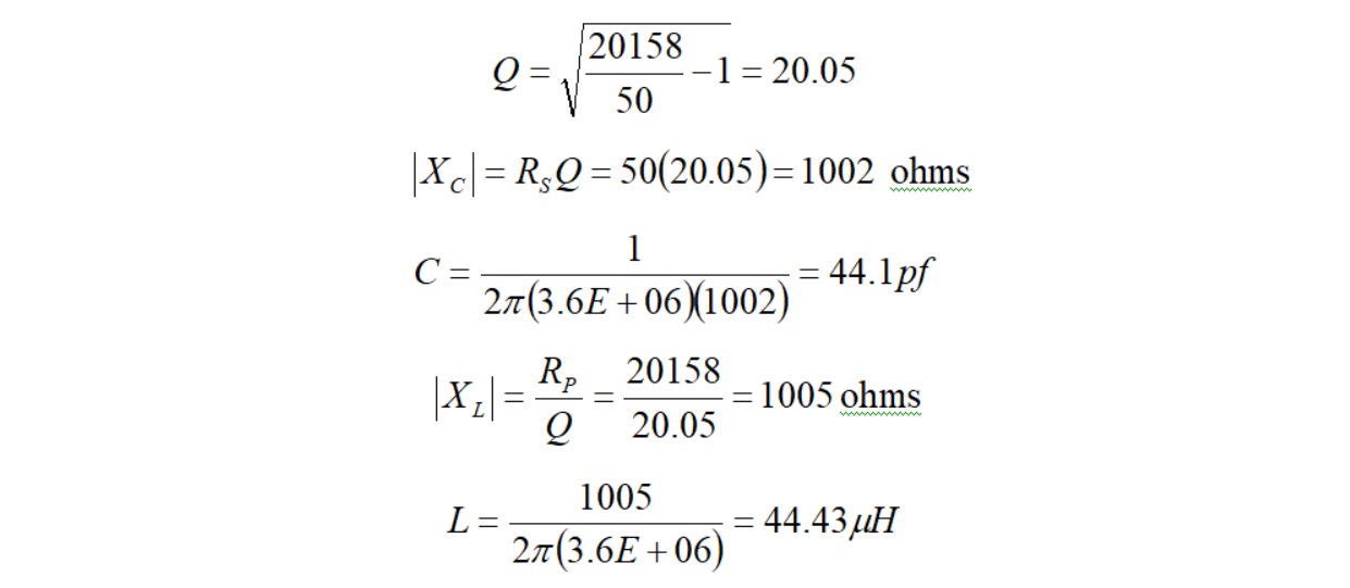
We make use of Figure 1(b) to compute the unloaded Q for the L-matching network

and

where
Substituting, we have

Also,


At 3.6 MHz, the matching network inductance is

and the matching network capacitance is

Step 2
Our matching solution is incomplete until we cancel the remaining part of the load impedance that we ignored earlier, i.e., the imaginary part of the load impedance,
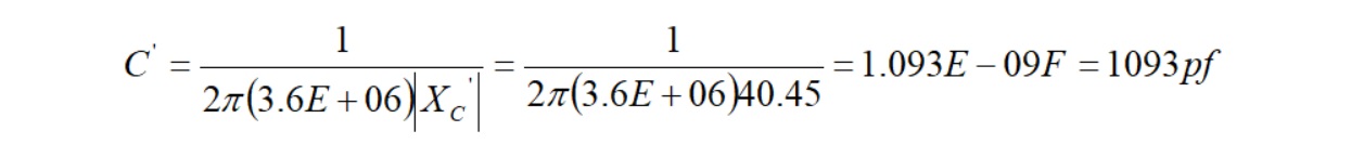
-j631.9 ohms, must be canceled to achieve a match. The secret to achieving a match is in finding a value of inductance that resonates with the capacitive reactance. Once completed, the series combination of load capacitance and added resonant inductance will result in zero reactance at the resonant frequency. We remember that for series resonance, ignoring any losses in the inductor and capacitor, the LC resonant pair looks like a short circuit at the design frequency. That’s exactly what we want – we want the load capacitance and the additional inductor to look like zero ohms at resonance. Of course, real inductors have series resistance due to the wire and capacitors have dielectric losses but for this exercise, we assume that they do not.
Thus, at resonance we have

where
C is the capacitance equivalent to the complex part of the load impedance, not the matching network, C‘, in units of Farads.
Thus,


The value, L”, is added to L‘. This will result in a new value for the L-matching network inductor, L”’

We don’t have to add the two together, and it may be easier to think about what each of the inductances does if we leave them as separate components.
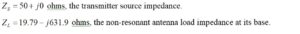
This matching circuit may be simulated using RFSim99[5]. The circuit model is shown in Figure 2. The inductors L‘ and L” are drawn separately for emphasis. (Two inductors in series may be added.)
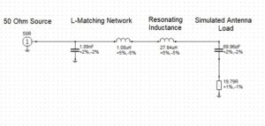
Figure 2. Low-Pass L-Matching Circuit. The inductor, L‘=1.08 μH, and added resonating inductor, L”=27.94 μH, are shown separately for clarity.
Return Loss and VSWR
In the VSWR section, above, we calculated the VSWR from

We may also calculate VSWR from the return loss, RL, directly from

where we have divided the return loss by 20 because the return loss is the voltage return loss.
Let’s calculate the VSWR for our simulation, where the return loss is 50 dB.

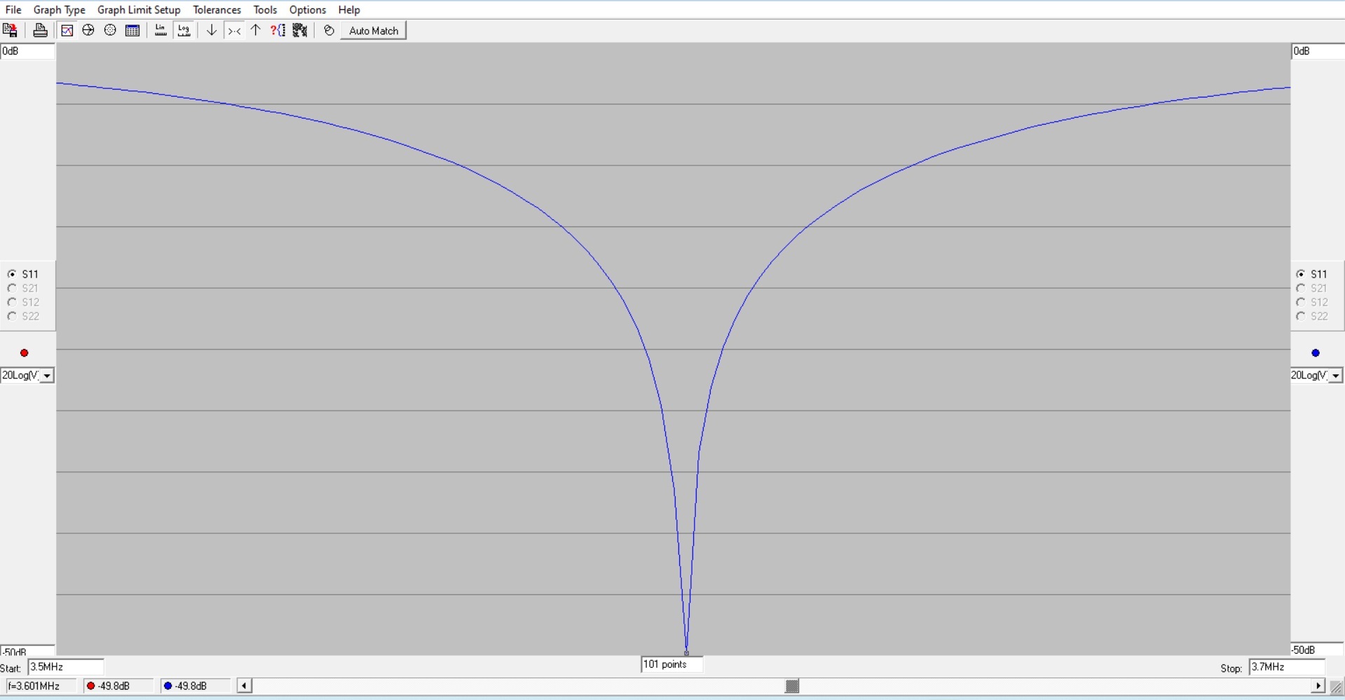
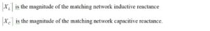
The resulting return loss for the low-pass matching circuit is shown in Figure 3. The 2:1 bandwidth of the matching network is ~78 kHz. The return loss is better than 50 dB at 3.601 MHz, or better than 1.01:1.
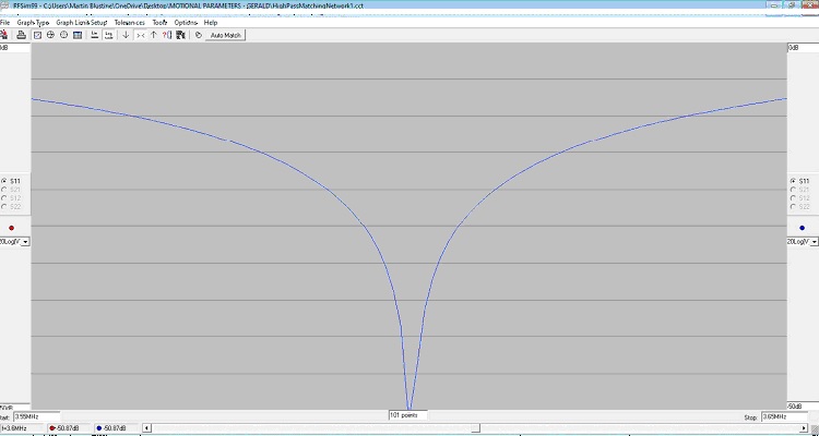
Figure 3. Return Loss for Low-Pass Matching Circuit. The 2:1 bandwidth of the matching network is ~78 kHz. The return loss is better than 50 dB at 3.6 MHz, or better than 1.01:1.
It may be concluded that this two-step matching technique for a low-pass matching network works quite well for our shortened antenna on the 80m band.
Example 2: High-Pass Topology with Series to Parallel Load Conversion
For the high-pass L-matching network Figure 1 shows that two topologies are possible. The one chosen would depend on how the capacitive reactance of the load is to be canceled.
There are two ways to accomplish this depending on where the inductance is in the matching network. The inductance in the high-pass configuration is always parallel at the input or parallel at the output. The position of the inductor depends on which is larger, RS or RL. The matching L-network inductor is always closest to the larger of the two as is seen in Figure 1.
The capacitance in the load is normally thought to be in series with the load resistance. This capacitive reactance could be canceled with a series inductor added to the L-matching network but there is a more interesting way to do it.
If the series RC load combination was converted to parallel form, as is often done for us on our VNAs, it would be observed that the new parallel resistance has a value that is much higher than the source impedance. By necessity, that would place the inductor in the high-pass L-matching network in parallel with the parallel capacitance of the load.
If we were to think about parallel resonance, and neglecting any losses in the load capacitor and resonating inductor, at resonance the pair looks like an open circuit. Then, the L-matching network just sees the real part of the load impedance.
The solution begins by converting the load from series form to parallel form.
Step 1
As it turns out, there is a transformation between series and parallel circuits that works at a single frequency. As was the case for the low-pass L-matching network, we ignore the reactive part of the load, initially. and incorporate it into the solution later. The series to parallel transformation works when

and

and

Then,

and

where
The Q-value is higher than we would like, but let’s proceed to see what happens.
There is enough information to derive the values

At 3.6 MHz the parallel load capacitance becomes

We observe that while the load resistance changes a great deal, the capacitance value hardly changes at all.
Step 2
Next, the real source impedance of the transmitter, 50 ohms, must be matched to the real part of the parallel load impedance. For this case we have determined by series to parallel transformation that

To keep our notation understandable, please note that for this section, RP is substituted for RL.
Since RP is greater than RS, we must use the correct high-pass equations for unloaded Q given in Figure 1(c).

Substituting, we find that
We have the values of capacitance and inductance that will match the pure 50 ohm source impedance to a 20158 ohm load resistance.
Step 3
Now it is time to resonate the parallel load capacitance that we calculated with a parallel inductor that will be added to our matching circuit. The value of this inductor will have a value that is similar to the one that we computed for the low-pass topology. We use the same equation for resonance as before

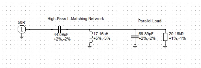
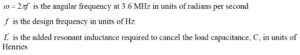
Figure 4 shows the model for the high-pass topology. A parallel inductor is introduced at the output of the L-matching network to resonate out the parallel capacitor in the load.
We don’t have to do it, but for practice, let’s go through the steps to combine the matching network inductor in parallel with the resonating inductor
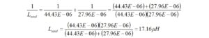
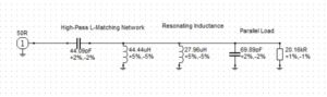
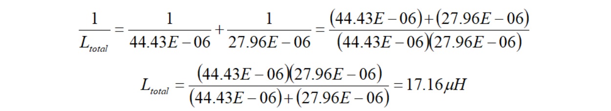
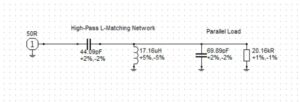 Figure 4. High-Pass L-Matching Network Topology. (Top) L-matching network with a separate resonating inductor as marked. (Bottom) L-matching network, where the L-matching network and resonating inductor have been combined in parallel to produce a single 17.16 μH inductance.
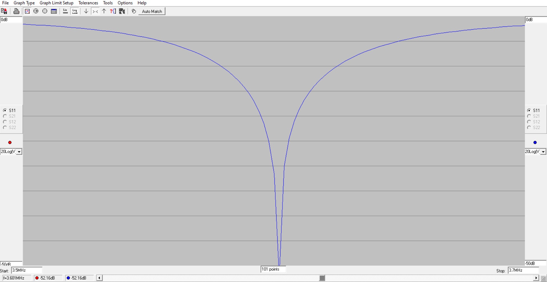
Once the simulation is run, Figure 5 shows that the high circuit Q results in a narrow 2:1 bandwidth, ~ 48 kHz. The 20158 ohm resistor is responsible for this.

Figure 5. High-Pass L-Matching Network Topology Return Loss. The return loss at 3.6 MHz is better than 50 dB demonstrating a VSWR of better than 1.01:1 over a narrow 48 kHz 2:1 VSWR bandwidth.
We conclude that the conversion to the parallel load configuration has resulted in an unloaded circuit Q that is high. This results in a narrower 2:1 bandwidth. The calculation is now repeated for the original series load to which will be added a series resonating inductor. Let’s see if the bandwidth can be improved.
Example 3: High-Pass Topology with Series RC Load
We return to the original series RC load impedance and choose the high-pass topology for the L-network.
Step 1
The high-pass solution for the series RC load begins with the following assumptions
The solution will ignore the imaginary reactance of the load impedance, initially. It will be used later.
The defining equations from Figure 1(d) for a high-pass L-matching network where the load resistance, RL, is smaller than the source resistance, RS, and where Q is the unloaded Q are given by

and

where
Substituting, we have


Also,

At 3.6 MHz, the matching network inductance is

and the matching network capacitance is

The value of unloaded Q is low, and the matching capacitance is high.
Step 2
The capacitive reactance of the load impedance has not yet been canceled as it was ignored in Step 1. A way must be found to cancel this reactance, but we observe in Figure 6 that the high-pass topology separates the load capacitance from the L-matching network shunt inductance, which is at the input.
Let’s try adding a series resonating inductance at the output of the L-matching network. That should work even though this inductance may not be combined with the L-matching network inductor.
The series load capacitance is resonated with a series inductor that will be added to our matching circuit. The value of this inductor is given by

The check for this topology is provided by the circuit model of Figure 6. A resonating inductance has been added in series with the L-matching network. It is not convenient to combine this series inductance with the parallel inductance at the input.
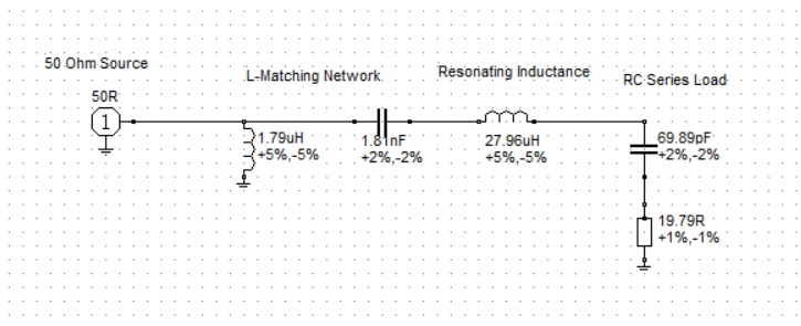
Figure 6. High-Pass L-Matching Network with Series Resonating Inductance Circuit Model. A resonating inductance is added in series with the L-matching network. It may not be combined with the parallel inductor at the input.
The results of this topology are shown in Figure 7. The return loss for this circuit model at 3.6 MHz is better than 49 dB for a VSWR or 1.01:1. The 2:1 VSWR is 78 kHz just as it was for the low-pass solution.
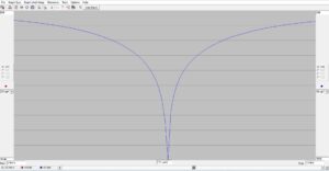
Figure 7. High-Pass L-Matching Network with Series Resonating Inductance Return Loss. The proof of this topology is evident from the plot. The return loss is better than 49 dB for a VSWR of better than 1.01:1 at 3.6 MHz. The 2:1 bandwidth is ~ 78 kHz which is the same as it was for the low-pass configuration.
The series RC load configuration is preferable over the parallel RC load configuration.
It may be concluded that this two-step matching technique for a high-pass matching network works quite well for the 80m band.
Conclusions
In Part I of this article we have used simple L-matching networks with additional resonating elements to match complex loads that possess capacitive reactance. This technique works for antennas that are too short. For antennas that are too long, the antenna load will also be complex but the resonating element required is a capacitor that cancels the inductive reactance of the complex load.
In Part II we will explore a different technique for matching to the complex load presented by a 43-foot backyard vertical antenna. The matching network will consist of a 1:1 UNUN followed by an autotransformer.
In Part III we will discuss the high voltages encountered in highly reactive loads. This occurs when antennas are far too long, or far too short.
References
[1] Salas, Phil, 160 and 80 Meter Matching Network for Your 43 foot Vertical — Part 2, QST, January 2010, pp. 34-37. http://www.arrl.org/files/file/QST%2520Binaries/QS0110Salas.pdf
[2] Ibid.
[3] Blustine, Martin, Highly Efficient L-Matching Networks for End-Fed Half-Wave Antennas, June 11, 2022. https://www.n1fd.org Add Contact Form /2022/06/11/l-matching-networks/
[4] Reproduced under CC BY-NC by permission from Michael Steer, North Carolina State University, LibreTexts™, 6.4: The L-Matching Network, https://eng.libretexts.org/Bookshelves/Electrical_Engineering/Electronics/Microwave_and_RF_Design_III_-_Networks_(Steer)/06%3A_Chapter_6/6.4%3A_The_L_Matching_Network
[5] RFSim99, Stewart Hyde, author, 1999. https://www.ad5gg.com/2017/04/06/free-rf-simulation-software/