Former Section Manager for the Colorado Section (2011-2020). Past President of the Boulder Amateur Radio Club (2002-2011). Former Emergency Coordinator for Boulder County ARES. Director and Co-Founder of the BARC Juniors Youth in Amateur Radio Club. Founder and Administrator of the BARC Scholarship Fund. Co-Founder and Member of Colorado Auxcomm. Member of the Mile High DX Association and Grand Mesa Contesters. Enthusiast in DXing, contesting, and emergency communications. For more about my life and experiences, visit my blog at wm0g.wordpress.com.
BATTERY LIFE CALCULATORTo calculate battery life, use the formula:
Battery life (amp hours) = Battery Capacity (amp-hours)
Current Draw (amps)
Battery life (amp hours) = 2.6 (amp-hours) / 0.135 (amps)
Given your battery’s capacity of 2.6 amp-hours and a current draw in the receive mode of 0.135 amps (135 mA), you can plug these values into the formula:
Battery Life (hours) = Battery Capacity / Battery Draw
Battery Life (hours) = 2.6 Amp-Hours / 0.135 Amps
Battery Life (hours) = 2.6 / 0.135
Battery Life (hours) = 19.26
With a 135mA current draw in receive mode, your battery will last approximately 19.26 hours.
For Example:
Elecraft KX2 Current Draw in Transmit Mode
The KX2’s current consumption during transmission varies based on factors like output power, operating mode (CW, SSB, DIG), and connected accessories. At 5 Watts Output Power (Typical QRP Operation):
• CW Mode: Draws around 0.8 to 1.0 amps. Considering a 25% duty cycle, the effective average current is approximately 0.20 to 0.25 amps.
• SSB Mode: Draws around 1.5 to 2.0 amps. With a 30% duty cycle, the average current falls between 0.50 to 0.70 amps.
• DIG Mode: Draws around 1.5 to 2.0 amps. Given a 65% duty cycle, the average current ranges from 0.98 to 1.3 amps.
________________________________________ At 10 Watts Output Power (Higher Power Operation):
• CW Mode: Draws around 1.5 to 2.5 amps. With a 25% duty cycle, the average current is approximately 0.38 to 0.63 amps.
• SSB Mode: Draws around 2.5 to 3.5 amps. Considering a 30% duty cycle, this results in an average current of 0.75 to 1.05 amps.
• DIG Mode: Draws around 2.5 to 3.5 amps. Due to a 65% duty cycle, the average current is roughly 1.6 to 2.3 amps.
________________________________________ Key Takeaways:
• Higher output power increases current draw proportionally.
• Digital modes (DIG) have the highest duty cycle, leading to greater average current consumption.
• CW and SSB modes, due to lower duty cycles, are more battery-efficient, especially at QRP levels.
Understanding these current draws and duty cycles can help you optimize battery life for portable operations. DUTY CYCLES – CW vs SSB vs DIG
The duty cycle of a transmitter refers to the percentage of time it actively transmits RF energy during operation. This varies significantly depending on the mode of transmission—CW, SSB, or digital. CW (Morse Code) Transmitters
For CW transmitters, the duty cycle during active transmission typically ranges from 10% to 30%. This is because Morse code involves alternating between brief periods of transmission (the dots and dashes) and silence (the spaces between characters and words).
For example, if you’re sending Morse code at a moderate speed of around 12 words per minute, with evenly spaced characters and words, the transmitter might be active for 1 to 3 seconds out of every 10 seconds. This results in an estimated duty cycle of roughly 10% to 30%.
However, this is only an approximation. The actual duty cycle can vary based on several factors:
• The specific Morse code being sent (longer dashes vs. shorter dots).
• The operator’s sending speed and technique.
• Pauses or breaks between transmissions.
________________________________________ SSB (Single Sideband) Transmitters
For SSB voice transmissions, the duty cycle is generally higher than CW but still relatively low compared to modes like FM or AM. This is because SSB transmits only when there’s audio input—primarily during speech.
The duty cycle for SSB typically falls between 20% and 40% during active voice transmission. This means that while conversing, the transmitter is active for part of the time when the operator is speaking, interspersed with silent periods between words, sentences, or pauses in conversation.
Factors influencing the SSB duty cycle include:
• Speaking rate and style (fast talkers vs. slow, deliberate speakers).
• The frequency and length of pauses.
• The nature of the conversation (continuous speech vs. short exchanges).
For digital modes over SSB (like FT8), the duty cycle can be much higher because data signals are more continuous compared to the sporadic nature of human speech.
________________________________________
Digital Mode Transmitters
Digital modes exhibit the widest range of duty cycles, depending on the specific mode and the data transmission pattern.
• High-Duty Cycle Modes: Modes like PSK31, FT8, and JT65 involve continuous data transmission in structured bursts, often with very minimal breaks. The duty cycle in these modes can approach 100%, meaning the transmitter is active almost the entire time during data exchange.
• Lower-Duty Cycle Modes: In contrast, modes like Packet Radio (AX.25) or APRS transmit data in discrete packets with intermittent breaks. The duty cycle in these cases is lower and varies based on:
o Packet size and frequency.
o Network activity and traffic load.
o Transmission settings and protocols.
________________________________________
Summary
• CW: 10% to 30% (depends on sending speed and style).
• SSB: 20% to 40% (varies with speech patterns and pauses).
• Digital Modes: Varies widely—from near 100% (FT8, PSK31) to much lower (Packet Radio, APRS).
Understanding these duty cycles is crucial, especially when considering transmitter cooling, power output settings, and overall equipment longevity.
No, I’m not talking about short people! I’m talking about hams who may not have tall trees or the capability to put up a tower on their property. I want to tell you about a fascinating antenna design – a low-profile, high-performance solution ideal for those of us who might be challenged by restrictive antenna regulations or limited space. I’m referring to the Magnetic Radiator, specifically the Multiple-U (MU) design detailed in this article. This clever design comes to us from the inventive mind of Paul D. Carr, N4PC (SK) who had a column in CQ Magazine many years ago.
Now, you might be thinking, “Another vertical antenna? What’s so special about this one?” Well, let me tell you. This isn’t your typical electric radiator. This antenna operates on a fundamentally different principle—it’s a magnetic radiator.
What does that mean? Electric radiators, like your standard dipole or vertical, generate a strong electric field close to the antenna, leading to ground losses and less efficient radiation. This design, however, focuses on creating a strong magnetic field, minimizing those losses, and improving efficiency. Think of it as radiating power through the earth rather than into it. Some key advantages of the MU design are:
Low Profile: The vertical elements are less than 0.1 wavelengths high, making it perfect for locations with height restrictions. We’re talking about an antenna that’s practical for even the most compact locations.
No Loading Coils or Radials: No need for cumbersome loading coils or extensive ground radial systems. This simplifies construction and installation considerably.
Efficient Radiation: The design promotes efficient radiation, even at relatively low heights above ground. This magnetic radiation pattern offers surprisingly good performance.
Good Bandwidth: The MU design offers good bandwidth, which is important for modern digital modes and for those who like to cover multiple frequencies in the same band without retuning.
The article provides details design specifications and construction guidelines for various bands, from 10 meters up to 160 meters, with diagrams to walk you through the process. It even offers adjustments for different antenna heights above ground.
Now, let’s be clear—this isn’t a magic bullet. The performance will vary depending on the specific location, and like any antenna, there will be some directional favoritism. In the examples provided, there is significant performance in a certain direction. However, the overall design offers impressive performance, considering its low profile and simple construction. Remember that the measurements presented are based on real-world testing, demonstrating its practical effectiveness.
If you’re looking for an efficient, compact, and relatively easy-to-build antenna that performs well for long-haul contacts, I highly recommend taking a closer look at the Multiple-U magnetic radiator. The provided charts and diagrams will help you determine your optimal design based on your specific band and location.
Back in the 1990s, I built this antenna on my four-acre property in Boulder, Colorado. Boulder County’s strict antenna regulations prevented me from using a tower despite having ample space. After extensive research, I chose this design and started with a 10-meter version, using readily available parts from my “junk box”—speaker wire and RG-59 75-ohm coax for the matching network. I improvised support using a nearby bush and my garden fence and constructed the antenna, including the spreaders, in under an hour.
Connecting my 50-ohm feedline to the quarter-wave 75-ohm balun, I was pleased to see my ATU quickly achieve a 1:1 SWR with minimal tuning effort—always a good sign. Using my old IC-745, I tuned into a busy pile-up on 10 meters. I cautiously sent my callsign, fully expecting nothing, especially with my low power output of only 100 watts. To my astonishment, the DX station from Malta immediately answered who was the reason for the pile-up.
This unexpected success initially left me stunned. After confirming the contact with a 59 report, he responded that my signal was 59+20dB at his location. I explained my simple antenna. He compared my signal to a friend’s using a 50-foot high tri-bander in Illinois, noting that I was significantly louder. Propagation undoubtedly played a role, but switching to my vertical antenna resulted in a noticeable decrease in his signal strength (about two S-units) – this proved to me the design was effective. I was hooked and decided to build a larger version for 80 meters.
Using four 25-foot supports, I constructed a much larger 80-meter version of the antenna, requiring approximately 530 feet of wire. Bamboo served as the spreaders, and a quarter-wave 75-ohm line provided the matching. I oriented the antenna east-west for broadside radiation. That evening, I monitored an 80-meter WAS net and was amazed by the clarity of the signals. Typically, 80 meters is noisy, but this antenna exhibited remarkably low atmospheric noise, a characteristic benefit of H-plane operation, which minimizes noise typically prevalent in the E-plane. The longer “skip” characteristic of this antenna meant that distant stations came in exceptionally well, making it ideal for DX but less effective for closer contacts.
I replicated the antenna design for another ham who wanted a directional antenna specifically for 17 meters. He lived in a trailer park with antenna restrictions, so we needed a lightweight, easily repositionable solution. We constructed two supports using PVC pipe, with a central section and two horizontal PVC spreaders at the top and bottom. To ensure stability, the base of the vertical PVC support was encased in cement, allowing him to easily adjust the antenna’s direction simply by moving the cement-filled buckets at the base of the supports, effectively changing the broadside direction as he desired.
The unexpected success of my initial 10-meter antenna, built from readily available materials and achieving exceptional signal clarity, fueled my curiosity for this simple yet effective design. The subsequent construction of larger versions for 80 meters and a modified model for 17 meters further confirmed its versatility and adaptability. These antennas, built to overcome challenging site restrictions, demonstrated the principle of H-plane operation in minimizing atmospheric noise while maximizing the reception of distant signals. The experience proved that resourcefulness, ingenuity, and careful design could significantly enhance signal quality in challenging operating environments.
You can learn more about magnetic radiator antennas here.
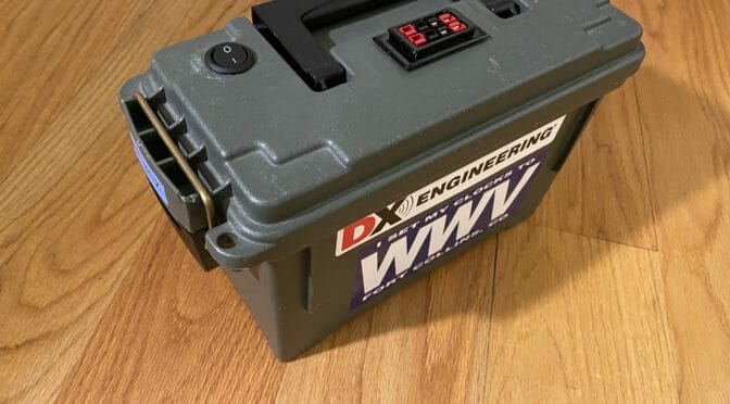
During our weekly Sunday night VHF net, a question arose about the National Institute of Standards and Technology’s (NIST) time and frequency station, WWV. Net Control asked, “When did WWV move to Colorado?” While a few of us could answer, it became clear that many of the newer hams didn’t know much about the WWV station.
Myself, being a ham from Boulder, Colorado and now living in Nashua, New Hampshire, I saw this as a great opportunity to share information I’ve gathered over the years, both about WWV’s operations in Fort Collins, Colorado, and its move from Maryland in 1966.
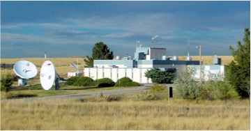
WWV Site – Fort Collins, CO
WWV is considered one of the oldest continuously operating radio stations in the United States. It was first established in 1919 by the National Bureau of Standards (now NIST) and originally broadcasted from Washington, D.C. Its primary purpose has always been to transmit accurate time and frequency signals, which it continues to do today from its Fort Collins, Colorado facility. WWV’s long history of broadcasting time signals makes it a significant part of radio history in the U.S.
Boulder, Colorado, is home to the NIST (formerly the National Bureau of Standards, or NBS) Atomic Clock, which serves as the time and frequency standard for the United States and many other countries around the world. I’ve had the opportunity to view the Atomic Clock “in person” at the NIST Laboratory.
The NIST atomic clocks use cesium atoms to keep incredibly precise time. Here’s a simplified explanation of the process:
Cesium Atoms: The atomic clock relies on the natural oscillation of cesium atoms. Cesium atoms absorb and release energy at a very consistent frequency when they transition between two energy levels.
Microwave Frequency: The clock generates microwaves that are tuned to match the exact frequency of the cesium atoms’ oscillation. The frequency at which cesium atoms oscillate is exactly 9,192,631,770 cycles per second.
Tuning to Maximize Accuracy: The atomic clock continuously adjusts the microwave frequency to ensure it matches the cesium atom’s resonance as precisely as possible.
Counting Seconds: By counting these highly accurate oscillations, the clock measures time. One second is defined as exactly 9,192,631,770 oscillations of the cesium atom.
Disseminating the Time: NIST broadcasts the official time using radio signals (via stations like WWV), the internet (through NIST’s network time protocol, or NTP), and satellite systems. These signals help synchronize clocks around the world.
NIST’s time standard is crucial for GPS systems, telecommunications, scientific research, and other industries that require precise timekeeping.
In 2013, when I was serving as the ARRL Colorado Section Manager, we hosted the Rocky Mountain Division Convention (Hamcon Colorado) in Estes Park, Colorado. Given its proximity to the WWV radio complex in Fort Collins, our committee thought it would be a great opportunity to arrange a tour for interested hams. Since WWV is a secure government facility, we needed special permission. The WWV Chief Engineer, who was also a ham, informed us that they had never conducted a tour before and it might be impossible, but he would ask. To our surprise, permission was granted with some necessary security measures in place. Interest in the tour was high, and we chartered a school bus to take a large group of hams to the facility.
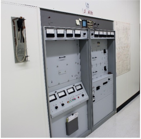
10 KW – 5 MHz WWV transmitter
The engineers at WWV went above and beyond, providing a comprehensive tour of the facility that included fascinating historical devices. We were able to visit the antenna sites and transmitters, with detailed explanations of their operations.
Historically, amateur radio operators played a key role in the technical development of the atomic clock and the WWV radio stations from their earliest days. Given that the atomic clock is housed in Boulder, CO, many members of the Boulder Amateur Radio Club (BARC) were among those who contributed to its development and advised on the WWV operations over the years.
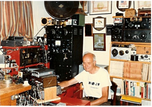
Yardley Beers, W0JF
ne of the more notable BARC members was Yardley Beers, WØJF (formerly WØEXS and W3 AWH), who earned his MS in Nuclear Physics in 1937 and a Ph.D. in 1941 from Princeton University, where Einstein was in residence at the time. Beers was a pioneering scientist who first utilized cesium as the core of the aforementioned time standard oscillator. He was a dear friend whose boundless curiosity, humor, and deep expertise in all things radio-related made him a wealth of knowledge for our club.
At 0000 GMT on December 1, 1966, the veteran time and frequency station WWV in Greenbelt, Maryland, shut down permanently. Almost simultaneously, a new station with the same call letters and services began broadcasting from Fort Collins, Colorado. The decision to construct the new station and relocate was driven by several factors, primarily the obsolescence of the old facility and significant maintenance challenges.
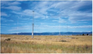
WWV 15-meter antennas
In contrast, the new station utilizes the latest transmitter designs, offering significantly more efficient operation. The setup also provides greater flexibility, as the transmitters consist of identical units—except for some higher-powered transmitters, which include an additional amplifier stage—that can be tuned to any frequency. At the old station, only a few of the eight transmitters were identical. Unlike the old transmitters, the new ones apply modulation at low levels, with all subsequent stages maintaining precise linearity. This allows for a wide range of modulation options, including AM or single sideband, with either sideband and any desired degree of carrier suppression. These features mirror those found in modern amateur radio transmitters.
Lastly, the move brings the benefit of administrative efficiency. WWV is now co-located with two other NBS standard frequency and time stations, WWVB (60 kHz) and WWVL (20 kHz), at the same site. Additionally, it is more convenient to synchronize the station with the NIST atomic standards, which are based in nearby Boulder, Colorado.
WWVH began operation on November 22, 1948, at Kihei on the island of Maui, in the then
territory of Hawaii (Hawaii was not granted statehood until 1959). The original station
broadcasts a low-power signal on 5, 10, and 15 MHz. As it does today, the program schedule
of WWVH closely follows the format of WWV. However, voice announcements of time
weren’t added to the WWVH broadcast until July 1964. In July 1971, the station moved to its current location, a 30-acre (12-hectare) site near Kekaha on the Island of Kauai, Hawaii.
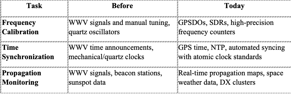
Today, the methods for calibrating frequency, synchronizing time, and assessing propagation have evolved significantly due to advances in technology, though some traditional methods (like using WWV) are still in use. Here’s a comparison of how these tasks were done in the past versus how they are typically done today:
1. Frequency Calibration
Before (Using WWV and Manual Tools):
WWV Broadcast: Operators tuned their radios to the exact frequencies broadcast by WWV (e.g., 5, 10, or 15 MHz) to verify or adjust their frequency dials
.Signal Comparison: Operators might use frequency counters or calibrate their equipment using signal generators. By manually adjusting their radio to match the WWV signal, they ensured their equipment was tuned correctly.
Crystal Oscillators: Some radios used quartz crystal oscillators that needed periodic manual adjustments to maintain frequency stability.
Today (Using GPS, Software, and SDRs):
GPS Disciplined Oscillators (GPSDO): Modern radio equipment can be calibrated with GPS, which provides ultra-precise time and frequency data directly from satellites. GPSDOs lock the radio’s oscillator to the exact frequency provided by GPS signals.
Software-Defined Radios (SDRs): SDRs can automatically lock to known reference frequencies or signals, often bypassing the need for manual calibration.
Digital Frequency Counters: High-precision digital frequency counters, often built into modern equipment, can accurately verify a station’s frequency without the need for an external signal like WWV.
2. Time Synchronization
Before (Using WWV or Manual Clocks):
WWV Time Signals: Operators would listen to WWV’s hourly time announcements and manually synchronize their clocks to the audio ticks or the minute mark. This ensured they had the correct Coordinated Universal Time (UTC) for logging contacts.
Mechanical or Quartz Clocks: Station clocks were either mechanical or quartz-based, requiring manual adjustments for drift.
Today (Using NTP and GPS):
Network Time Protocol (NTP): Computers, logging software, and transceivers are often synced to the Internet time servers using NTP, which automatically keeps time to within milliseconds of UTC. Many hams now use computers with built-in NTP syncing for contest logging and communication accuracy.
GPS Time: GPS provides highly accurate time synchronization. Many modern radios or station computers are connected to GPS receivers that provide time directly to within a fraction of a second of UTC.
Atomic Clocks: Although not widespread in amateur radio, some operators use atomic clock-based devices for extreme precision in timekeeping, often integrated with GPS.
3. Propagation Monitoring
Before (Using WWV and Beacons):
WWV Propagation Monitoring: Hams listened to WWV signals on different frequencies (2.5, 5, 10, 15, and 20 MHz). The strength of the signal provided a rough estimate of how well certain bands were propagating, helping operators decide which frequencies to use.
Beacon Stations: Operators tuned to beacon stations operating on different frequencies around the world. By monitoring when these signals were heard, they could get a sense of global propagation conditions.
Sunspot Numbers: Many hams used published sunspot data and predictions to estimate the effectiveness of different HF bands.
Today (Using Online Tools and Real-Time Data):
Real-Time Propagation Maps: Websites and apps like PSKReporter, DXMAPS, Reverse Beacon Network (RBN), and WSPRnet provide real-time data on where signals are being received and which bands are open. These platforms track signal reports and provide a visual display of current propagation conditions.
Solar and Geomagnetic Data: Many hams now use online services that provide real-time solar flux, geomagnetic indices, and space weather data. Websites like Space Weather Prediction Center (SWPC) offer detailed insights into how solar activity is affecting the ionosphere.
Cluster Networks: DX cluster networks provide real-time information on stations spotted around the world, giving hams direct feedback on current band conditions.
Software Tools: Advanced propagation software like VOACAP or HamCAP allows operators to model HF propagation based on real-time data, including solar activity, time of day, and location.
Summary of Key Differences:
While older methods like WWV are still valuable, modern technology has automated and refined many of these tasks, making it easier and more precise for amateur radio operators to ensure their equipment is accurate and their communication effective.
We use cookies to ensure that we give you the best experience on our website. If you continue to use this site we will assume that you are happy with it.