All posts by Dave Michaels

Yagi Antenna Teaching Construct Part #3: Directional Gain and Front to Back Ratio

In this final article of our series on the “Lego-style” antenna for teaching basic antenna physics and behavior, our focus is a Yagi-Uda 3-element antenna for 2 meters. The Yagi antenna is the most common construction form for a “beam” antenna. The Yagi has high gain in one specific compass (azimuth) direction and very low gain in the opposite direction when compared to the classic 1/2 wave dipole. The Directional Forward Gain and “Front to Back” Ratio (F/B Ratio) features are hallmarks of the Yagi and the reasons for its high popularity. The forward gain dramatically increases “Effective Radiated Power” in a chosen direction; the Front to Back Ratio dramatically reduces interference from signals to the antenna’s backside.

BASIC PRINCIPLE OF THE 3-ELEMENT YAGI ANTENNA

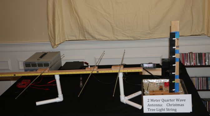
The Yagi antenna shown in the Feature Picture above has 3 radiating elements. The center element (with the coax attached) is the “Driven Element” (DE) receiving RF energy from the transmitter.  The other two elements are “parasitic”, meaning they are not connected to the transmitter. These elements absorb energy from the DE RF wave and re-radiate it by Faraday’s Law of Induction. This fact gives both parasitic elements a 180-degree phase shift relative to the DE. In the above picture, the left side element is the Reflector, typically 5% longer than the DE; the right side element is the Director, typically 5% shorter than the DE.  The length differences make both elements slightly off resonance to the DE RF wave which adds a second phase shift relative to the DE. Finally, the distances on the boom between the DE and parasitic elements adds a third phase shift since it takes a finite time for the DE wave to reach the Reflector and Director.  The distance between the DE and the parasitic elements vary between 0.1 to 0.25 wavelengths depending on materials, construction details and design goals for the forward gain and F/B Ratio.

The Yagi secret is that the sum of these three phase shifts for the 3 elements add in a way that reinforces each other for RF energy moving towards the Director. However, RF waves moving towards the Reflector combine in a way that subtracts and leaves little RF energy.

Figure 2 provides an illustration of this action using only waves interacting between the DE and Director, for simplicity.

Yagi Antenna PhasingFigure 2.  Summing RF wave from the Driven Element with the Induced wave from the Director Element (from Wikipedia, Yagi-Uda Antenna)

The DE RF wave (in green) reaches the Director parasitic element and induces a second RF wave (in blue) by Faraday’s Law. The multiple phase shifts that make up the Director RF wave gives a forward moving emission that adds to the DE wave yielding a combined larger RF wave.  However, the Director RF wave moving back towards the Reflector is nearly 180 degrees out of phase to the DE wave and the two nearly cancel each other out.  A similar analysis at the Reflector element shows that Reflector waves moving towards the DE and Director also adds to their waves to create an even larger wave. However, Reflector waves traveling off the rear of the antenna subtract with waves arriving from the DE and Director yielding very little RF energy leaving the backside direction of the antenna.

THE TOOLBOX FOR OUR EXPERIMENTS

The top Feature Picture shows the “Lego-Style” antenna in a Yagi assembly and the Lamp Bridge Receiver ½ wave dipole antenna is seen in the upper right corner. The Lamp Bridge Receiver lights when resonant RF is sensed and we used this tool in both Parts 1 and 2 of this article series.

New to our toolbox is a breadboard circuit to measure RF power in a semi-quantitative way using an LED Bar Graph display. The breadboard was built on an Analog/Digital Trainer Module and is seen in the lower right corner. The circuit samples the RF signal received by a 1/4 wave antenna (black antenna seen behind and above the breadboard). The induced RF current is converted to a dc voltage that feeds to a 30-stage linear increasing voltage comparator circuit.  A comparator turns on an LED when its voltage threshold value is reached. Our circuit is using only 15 LEDs due to breadboard space limits; however, by skipping every other comparator we are still measuring a 30 fold signal range. The picture shows 3 lit LEDs indicating a sensed voltage that is one-fifth the dynamic range of the circuit.

EFFECTIVE RADIATED POWER: COMPARING THE DIPOLE and YAGI-UDA ANTENNAS

A)  BASIC DIPOLE PERFORMANCE

We will use the classic 1/2 wave dipole as the benchmark to assess benefits of the 3-element Yagi-Uda antenna.  We begin by measuring relative radiated power of the dipole as we increase transmitter power stepwise between 5, 10, 20 and 40 watts.  The power detector circuit consists of a standard 1/4 wave stub antenna connected to the LED Bar Graph RF meter.  The results will be used to “calibrate” the detector circuit and be our reference point when we calculate Yagi Gain.

The video below explains the use of the LED Bar Graph RF meter; then it shows the actual testing protocol and you can see the LEDs report received RF signal as we increase Tx power to the dipole.

The results of received RF signal versus transmitter power for the dipole antenna are summarized in Table 1.  The data show a close to linear correlation (as expected) within the semi-quantitative limits of the Bar Graph Display.


Display Calibration

B)  3-ELEMENT YAGI PERFORMANCE

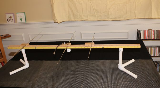
The next video shows the antenna forward radiated power as we stepwise build the Yagi beginning with the basic dipole; the addition of the Reflector element and a third addition of the Director element.  Note, the Tx power is constant at 5 watts.  Details of the Yagi construction (element lengths, spacing, etc.) are given in the video.

The data for the RF radiation received with the stepwise addition of elements to assemble the YAGI antenna are summarized in Table 2.

Yagi Antenna ERP

There is a significant increase in antenna forward received signal (looking towards the direction of the Director) as we add the two parasitic elements.  The signal increases by 3+ fold with the Reflector over the dipole and then by 7+ fold for the combination of Reflector plus Director. However, we want to translate the results to customary power level values in decibels.  The combined data of Tables 1 and 2 let us do this as an estimate of Directional Forward Power.

Gain for 2-Element  Antenna in dB:
7 Lit LEDs at 20 watts for dipole and 5 watts  for Yagi
dB  =  10 x Log(20/5)  =  6.0 dB  (= 1 S meter unit)

Gain for 3-Element Yagi in dB:
15 Lit LEDs at 40 watts for dipole and 5 watts for Yagi
dB  =  10 x Log(40/5)  =  9.0 dB  (= 1.5 S meter units)

THE FRONT TO BACK RATIO OF EFFECTIVE RADIATED POWER FOR THE 3 ELEMENT YAGI ANTENNA.

A)  THE 1/2 WAVE DIPOLE

We begin our experiments on Front to Back received power using the basic 1/2 wave dipole as we did above for forward radiated power.  However, since the dipole is symmetric side to side we will label our measurements as “left side” and “right side” to the wire axis. Second, our dipole experiment will use the Lamp Bridge Receiver antenna because we will use power levels not requiring amplification (the LED Bar Graph RF meter has a 10x gain built-in). Also, resetting the LED RF meter at the opposite table end is not easy.

The 2-sided picture below shows the responses of the Lamp Bridge Receiver antenna to a 40-watt transmission.  Picture 1A shows the received signal on the left side of the dipole; Picture 1B shows the response on the right side of the dipole.

Yagi Antenna Pattern

As you would expect, the radiated power of a basic 1/2 wave dipole appears equal broadside to the wire axis, as we learned in the Technician License Class.

B)  The 3-Element YAGI-UDA Antenna.

Our last video has a simple experiment showing the Front to Back Ratio effect of the Yagi antenna for radiated power parallel to the boom axis.  We return to using the LED Bar Graph RF meter for the experiment. The study is made easy by the simple trick of swapping placement of the Reflector and Director elements, a benefit of the “Lego-Style” construction of our antenna model.         

The study results are striking.  The data for the Forward RF signal from the Yagi showed an 8x fold increase over the basic dipole with 15 lit LEDs at 5 watts for the Yagi versus the dipole needing 40 watts to elicit the same response. We also saw this result in Video 2 (compare data in Tables 1 and 2). In contrast, the received Back-Side RF signal gave only 1 lit LED.  The difference merits visual repetition with a paired picture display.

Yagi Antenna Pattern

We can transform this data to estimate dB Power Gain of the Back-Side signal in a similar fashion as the Directional Forward Gain.  Again, we use data from Tables 1 and 2.  However, we need to interpolate the signal response of the Yagi Back-Side signal of 1 LED with the 2 LED response for a dipole at 5 watts. The factor is 1/3, not 1/2. Why?   Remember, the RF detector circuit divides the received signal into 30 equal size buckets, but we only look in every other bucket with an LED.  Hence, LED #2 measures the third bucket, not the second bucket.   I will repeat the Forward Gain calculation here to make the result comparison easier.

Forward Gain for 3-Element Yagi in dB:
15 Lit LEDs at 40 watts for dipole and 5 watts for Yagi
dB  =  10 x Log (40/5)  =  9.0 dB   (1.5 S meter units)

Backside Gain for 3 Element Yagi in dB:
1 LED (Yagi) = 1/3 (5 watts) =1.7 watts
dB  =  10 x Log (1.7/5 )  =  –  4.6  dB

We now can easily calculate the Yagi Front to Back Ratio:
F/B Ratio  dB  =  9.0  dB  –  (-) 4.6 dB  =  13.6  dB
(Remember, dB is a logarithm value, so we subtract the 2 numbers, not divide them)

C)  Results Analysis

The result of 9.0 dB for Yagi Forward Gain is likely high considering an expected typical range of 6 to 8 dB (seen in commercial units).  The estimate for the F/B  Ratio of 13.6 dB seems low, again based on typical commercial units that can have an F/B of about 20 dB.  However, the cited values are for “Far Field — Free Space” conditions; conditions not simulated in a 20 x 20 ft. room in my house.  Also, the experiments made no effort to optimize Forward Gain or the F/B Ratio by element lengths and spacing.

The list of experimental error sources in our studies are many; a partial list includes detector circuit layout that combined RF, digital and DC signals on one board, the accuracy and precision limits of discrete LEDs, antenna height above ground issues and wall-plus-apparatus surfaces that both absorbed and reflected RF signals.

Still, the “Lego Style” Yagi Antenna Assembly permits an easy way to demonstrate many basic antenna properties while showing performance results that are reasonable.  Perhaps, the next ham adventurer to design Version #3 will expand experimental versatility and improve performance areas.

I hope this series of three articles has expanded antenna knowledge to newly minted hams and has re-kindled interest in antenna experimentation for more experienced hams (many more knowledgeable than me).  Coming full circle to my thoughts as I began this article series, our antennas are the magic carpet that we ride over the airwaves whether to friends across town or to that rare DX station 10,000 miles away.  Enjoy the Ride!

I owe a heartily thank you to Skip Youngberg (K1NKR) for reviewing my draft manuscript for Part #3 and contributing valued suggestions. Also, the complete series of three articles could not have happened without the multi-media assistance, encouragement and full support from a special YL, Teresa Mendoza.

73,

Dave N1RF

Yagi Antenna Construct Part #2: Current, Voltage Profiles, and Dipole Pattern

In Part 1 of this article series, I presented the “Lego” 2 m 3-element Yagi antenna design that the N1FD ham license teaching team has used over the past year for class demonstrations.  The design allows easy assembly of the basic dipole antenna as well as a 3 element Yagi. The configuration of individual elements and spacing between elements can be quickly changed to demonstrate basic physics and behavior of these popular antennas.

The first article described antenna construction details and showed how to demonstrate the criterion for resonance as well as the polarization property of the radio wave.  In Part 2 of the series, I will continue a focus on the dipole, specifically the spatial current – voltage profiles on the driven element and the radiation pattern of the antenna.  We will use this information in Part 3 of the series next month to demonstrate how a 3-element Yagi works and why it is so popular.

THE CURRENT & VOLTAGE PROFILES ON A HALF WAVELENGTH DIPOLE   

Current Profile on a Half Wave Dipole Antenna
Figures 1a and b – Current Profile on a Half Wave Dipole Antenna

Figure 1a reminds us of the basic dipole geometry; and Fig. 1b shows the current and voltage profiles along the driven element.  (From http://www.radio-electronics.com/info/antennas/dipole/half-wave-dipole.php)

Note from Fig. 1b that the current profile of a dipole has a maximum current level at the center feedpoint and decreases to zero current at the end of each element arm.  Contrasting, the voltage profile has a zero value at the feed point and increases to a maximum level at the ends of the element arms.

1/4 Wave Vertical. Note the 7 spaced lamps.
Figure 2 – 1/4 Wave Vertical. Note the 7 spaced lamps.

The 1/4 wave vertical antenna seen in Figure 2 can be used to visualize the current profile along the arms of a 1/2 wave dipole.  The 1/4 wave antenna is made from a short length of a Christmas tree (incandescent) light string.  The string length can be estimated from the standard equation:  Length (ft) = 234/Frequency in MHz. Generally, several inches needs to be trimmed off because the lamps add “electrical length”. The shown antenna has the same resonance frequency as the Lego Style dipole we will use later (i.e., 146.550 MHz). The top end of the antenna is marked by the blue tape immediately above the 7th lamp.

Transmitting mode. Note pattern of lit and unlit lamps.
Figure 3 – Transmitting mode. Note pattern of lit and unlit lamps.

The energized antenna with 15 watts RF signal is seen in Figure 3.  Compare the pattern of lit and unlit lamps with the current profile sketch shown in Fig. 2b.  The three lamps, counting from the picture bottom are brightly lit from an RF current.  Lamps 4 and 5 show progressed less light indicating a lower RF current.  Lamp number 6 is barely lit and number 7 is dark indicating together very little to no RF current at the element top end.  The light pattern is a clear mimic of the diagram in Figure 1b.

Demonstration of the Voltage and RF Radiation Profile on a Half Wave Dipole Antenna

The voltage profile on a center fed 1/2  wavelength dipole is seen in Figure 1b. As mentioned above, the voltage is zero at the dipole center and increases in monotonic fashion to a maximum value at the antenna ends.

Illustration of Dipole RF Radiation Pattern
Figure 4 – Illustration of Dipole RF Radiation Pattern

The familiar RF radiation pattern of a dipole is shown in Figure 4 (taken from the cited source for Figure 1).

We are all well-schooled on the pattern, so I will just list the three key facts.  First, the RF radiation is broadside to the antenna axis. Second, the RF field intensity is equal on the left and right sides of the dipole axis (i.e., there is no discerned “front to back” sidedness. Third, there is (theoretically) no RF radiation off the ends of the dipole wire.

The dipole voltage profile and the RF radiation pattern can be demonstrated using the basic dipole element of our “Lego Style” antenna and two simple tools. The voltage profile, or more correctly, the electric field strength around the dipole is sensed by a small fluorescent light tube.  The actual RF radiation from the energized dipole is sensed by the flashlight lamp-bridged receiver antenna introduced last month in Part 1 of this series.

  1. Direct RF Radiation Visual Detection

The video below (double-click in the picture box) demonstrates the use of the lamp-bridged receiver antenna to detect radiated RF power.

The video shows the flashlight bulb bridging the handheld receiver antenna lights up when it detects an RF signal that matches its resonance point at 146.550 MHz  The light bulb is dark with no transmitted RF power from the Lego dipole. Keying the radio energizes the Lego dipole and the receiver lights up about equally on the right and left sides of the Lego antenna.  This reflects the figure 8 pattern of RF power illustrated in Figure 4.

  1. Voltage Profile witnessed by the Electric Field Strength.

The next video (double-click in the picture box) employs the fluorescent light bulb to map the voltage profile along a dipole arm by sensing its electric field strength.  An RF electric field causes a series of chemical reactions within the light bulb that produces a bright fluorescent light.

The light bulb is dark when the Lego dipole is not transmitting an RF signal. Keying the radio generates an RF signal and the associated electric field around the dipole element causes the bulb to light up. Note, the bulb is very bright adjacent with the side end of the dipole arm and extinguishes as it is moved to the dipole centered feedpoint. Also, the light is dimmed at the antenna tip in-line with the dipole axis.

The voltage profile map seen in the fluorescent light bulb video augments the RF signal map seen in the lamp-bridged receiver antenna video.  Also, it extends our demonstration to the expected observation that there is (theoretically) no RF radiation off the end tips of dipole elements.

CONCLUSION 

In this second installment of our Lego-Style Antenna series, we have shown how this construct together with two simple tools can be used in the classroom to demonstrate basic properties of the ubiquitous dipole antenna; Namely, criterion of resonance, generation of RF radiated waves, the polarization of the RF field (horizontal or vertical) and the general propagation geometry of these waves relative to the antenna orientation.

In Part 3 and last installment of this series we will continue to use the Lego-Style Antenna in its’ Yagi configuration together with the two accessory tools to show how properly designed and placed reflector and director elements on the Yagi antenna can shape and control the dipole rf signal to increase gain via spatial directivity  and improve signal selectivity by the “front-to-back” ratio that it creates.

73 & Hope to hear you on the air,

Dave N1RF

Hands-On Yagi Antenna Construction 2.0 for Teaching and Experimentation

The most important piece of equipment in ham radio is our antenna.  We are connected to the world with the magic of radio waves!  Each License Exam from Technician through Extra class has questions to test our knowledge on antenna design and building skills.  Home-brewed antennas are easy and relatively inexpensive projects.

This article describes a 2m, 3-element Yagi antenna construction concept that the N1FD FCC license teaching team has used over the last year for class demonstrations.  The “Lego” style construction (v. 2.0) shown in the above picture is our new design that demonstrates the operating principles of the ubiquitous basic dipole antenna as well as a 2-meter, 3 element Yagi.  (Note, This project evolved from an earlier effort by Diana Eng at Makezine.com, which can be seen here.

In this Newsletter issue, we will describe the construction of the “Lego” stylized antenna and show how it can illustrate basic properties of a dipole antenna.  We will build a Yagi antenna with the addition of reflector and director arms in a future Newsletter article.

CONSTRUCTION of the LEGO STYLIZED ANTENNA.

Yagi Antenna - Lego Antenna Parts and Receiver Antenna
Lego Antenna Parts and Receiver Antenna

The antenna demonstration unit consists of two assemblies. 

  1. A handheld receiver dipole set to a fixed frequency (e.g., 146.550 MHz). It is shown at the top of the photo above. It follows a “plumber’s delight” construction using pieces of PVC pipe for a short boom and handles.  The dipole arms are two telescoping (7-28 inch) FM radio replacement antennas, available on eBay or Radio Shack ($4-6 dollars).  The arms feed through the boom and are epoxied.  Bridging across the arms is a common 6-volt flashlight bulb.  The bulb lights up when the dipole receives a resonant rf signal.
  1. The “Lego stylized” Yagi antenna components are shown below the receiver unit. The boom (middle item) is made of red oak dimensioned at ¾  x  1 ½   x  48    The top surface is grooved to hold an epoxied  3/16  steel rod.  The bottom surface has drilled recesses to fit ¾ in PVC pipe for leg stands. The edge of the boom has two 24-inch adhesive tape rulers running from center to front and back of the boom.  The rulers read-out the spacing between the driven dipole element and the parasitic reflector and director arms. In the photo, the D.E. and parasitic elements are seen below the 48 in. boom.  The center element is the driven dipole and it is flanked by identical units that can be configured as either reflectors or directors.   Each unit consists of two telescoping FM radio antenna rods epoxied in a grooved piece of red oak ( ¾  x  1 ½  x  3 inches) serving as “riders” on the boom.  The telescope arms can be adjusted to “resonance” at any frequency in the 2-meter band. The bottom of all riders has 2 x ½ inch rare earth magnets.  These allow the three antenna elements to be fixed at any position on the 48 in. boom.

You can view a closer look at the assembled Yagi antenna configuration in this video (Click on Link)

DEMONSTRATIONS OF BASIC DIPOLE BEHAVIOR. 

1.  Antenna Resonance Determined by Dipole Length.

As we all know, the resonance length of a dipole is given by the equation:    L (in inches)  =  5616/ [ Frequency (in MHz)].  We can show this fact with aid of the “receiver” antenna, which is set for a frequency of 146.55 MHz  The light bulb of this antenna will light when it senses a signal of this value from our “Lego” antenna.

In the video below (Click on Link), we begin with a resonant D.E. length of 38.5 inches and see the receiver antenna light up.  Next, we manually shorten the D.E. and see the bulb light dramatically dim.  When the D.E. length is returned near the start value, the light bulb again brightens up.

  1. Effect of SWR on Signal Strength.

Most modern transceivers have a built-in auto-tuner that can match SWR up to 3:1.  We know this only makes the “radio happy”, still we key down without much thought on how our Tx signal degrades with a 3:1 match.  The pictures below use the transmitting “Lego” dipole and receiver dipole to show the received signals for an SWR of 1.1 and 3.0.  The SWR was changed by lengthening the D.E. elements by 2 inches while holding the Tx frequency at 146.55 MHz

Yagi Antenna - Receiver Signal-for Lego Dipole SWR 1.1
Receiver Signal-for Lego Dipole SWR 1.1
Yagi Antenna - Receiver Signal- for Lego Dipole SWR 3.0
Receiver Signal- for Lego Dipole SWR 3.0
3.  Polarization Effects between Tx and Rx Antennas.

A horizontal dipole shows “horizontal” polarization; meaning the electric field vector of the rf signal is parallel to the earth surface.  Similarly, a vertical dipole displays “vertical” polarization with the electric field perpendicular to the earth. We all learn this in a Technician class course.

When we use our 2m HT’s for short distance contacts, Tx and Rx antennas with opposite orientation create a huge signal loss.  The effect is shown dramatically in the video below.

CONCLUSION 

Our classroom constructible antenna for demonstrations in our Ham Radio license classes has evolved in design over the past year.  We believe it has been a useful resource,  helping students translate textbook theory to “Hands On” practice.  Perhaps, this review has kindled interest for our readers to think of their Next Antenna Project!

73 & Hope to hear you on the air,

Dave N1RF

Radio Amateurs Developing Skills Worldwide