Introduction
Out of curiosity I recently downloaded a copy of RFSim99[1], authored by Stewart Hyde, to see what it could do and how easy it was to use. It runs as a standalone app. This is a very old program and much to the credit of the Gordon Hudson, AD5GG[2], an extracted version seems to run on Windows 11 in compatibility mode for Windows XP.
There were some posts online about how some of the user interface buttons would not appear until hovering the mouse over where the buttons should appear[3]. Another quirk had to do with plots not appearing after the simulation button was pressed. I encountered both of these quirks when I first installed the application, particularly after I had run my first simulation. After unzipping the program for a second or third time, I ran a Sample File from the Open file menu. It ran with no problem whatsoever. Next, I created a circuit model of my own, saved it and ran a simulation. This time everything worked and continues to work, as it should. If all else fails, you could try to alter the compatibility settings that may be found under Properties by right clicking the RFSim99 icon. I changed the settings to a later version of Windows XP. It is a good idea to save all circuit model files in a folder apart from the app in the event the program file folder has to be overwritten.
This application is highly intuitive and can be up and running in minutes. If you wish to rotate or flip a component, all you do is selected it and hit the space bar. The easiest way to correct an error is to select the mistake and hit delete on the keyboard.
Three simulations are the subject of this article; a 40m L-matching network for an EFHW antenna, a 2nd harmonic optimized lowpass filter and a Butterworth bandpass filter. These demonstrate different plotting features that are available in RFSim99; Smith Chart plots and rectangular plots, respectively.
This simulation app is very useful because it can return a full set of S-parameter results. We can derive anything and plot everything from the data set.
Simulation of a 40m L-Matching Network for EFHW Antennas
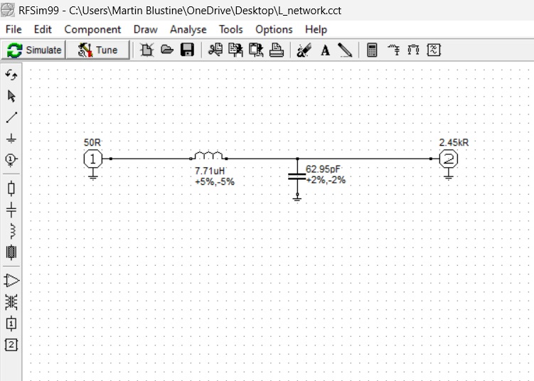
I decided to begin by running a simulation on a 40m L-matching network. These networks were the subject of an earlier article[4]. The matching network to be simulated is shown in Figure 1. A 50-ohm source drives an L-matching network that employs a lowpass topology. It is lowpass because the inductor is in series, and it will pass DC from input to output. A match from 50-ohms to 2450-ohms is required to match the high end impedance of an End-Fed Half-Wave (EFHW) antenna. Many of you will recognize this impedance transformation as being equivalent to the transformation performed by a 1:49 transformer. The design frequency used for the L-matching network was 7.15 MHz.
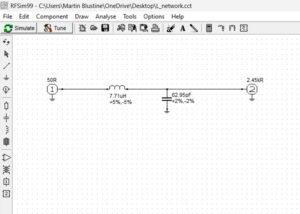 Figure 1. A 40m L-Matching Network. The lowpass topology is designed to match a 50-ohm transceiver to the 2450-ohm end impedance of an EFHW antenna at 7.15 MHz. The lowpass topology can be identified by the series inductor that can pass DC from input to output. Please note that there is a shunt capacitive element closest to the load. That means that this network is capable of transforming a higher load impedance down to a lower source impedance.
The results of the simulation are plotted using the Smith Chart option shown in Figure 2 that is available from a pull-down menu after running the simulation. The Smith Chart is simply a rectangular plot of real (resistance) and imaginary (reactance) values that has been cleverly constructed so that the reactance axes at infinity in the complex plane touch at the right hand side of the chart. It is an ingenious way of plotting axes that are infinite on a single sheet of paper. In order to do this the real resistance axis becomes more compressed to the right hand side of the chart, too.
If you are not familiar with Smith Charts, all of the values on the chart have been normalized to unity at the center of the chart. That makes it possible to use the chart to represent different characteristic impedances including 50-ohms. To get the final answer, we just multiply the number or numbers on the chart by the characteristic impedance. There is a cursor-slider on the bottom of each plot in RFSim99 that reads out the cursored values to the left and right sides of the chart. That is why there are no numbers displayed on the Smith Chart, itself.
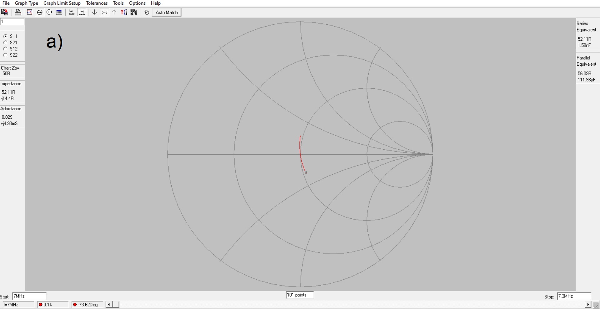
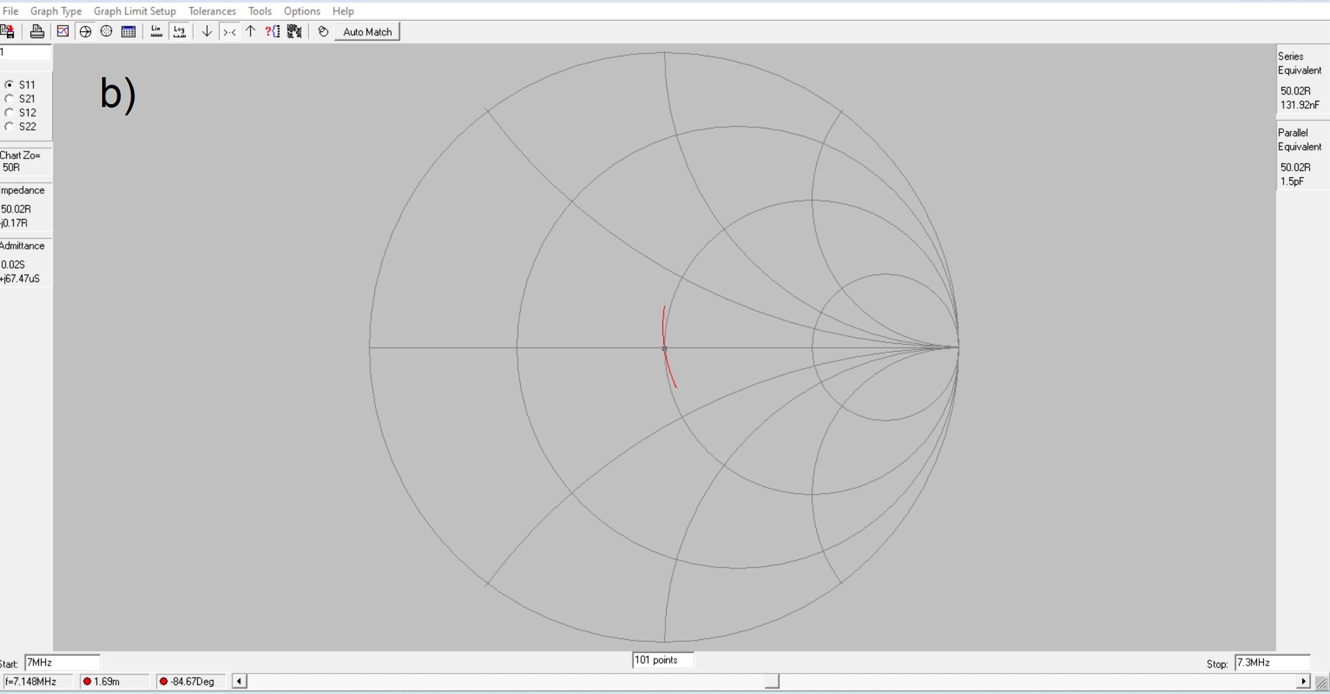
Figure 2 consists of three plots at three different frequencies, 7.0 MHz, 7.15 MHz and 7.3 MHz, respectively. Since our antenna is too short at 7.0 MHz, the plot at a) exhibits capacitive reactance of ~14-ohms. At b) for the design frequency of 7.15 MHZ the antenna length is resonant and nearly zero reactance is exhibited. At c) for 7.3 MHz the plot exhibits inductive reactance of ~14-ohms because the antenna is too long. Please note that the impedances and admittances displayed to the left of each plot correspond to the position of the cursor. The series and parallel equivalent circuit values are displayed to the right of each plot.
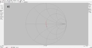
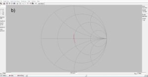
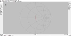
Figure 2. Smith Chart Plots of L-Network Impedance. The upper half of the Smith Chart plots inductive reactance while the lower half of the chart is capacitive reactance. The horizontal axis plots resistance with 50-ohms at the center of the chart. Please note where the cursor is and where the impedances are displayed to the left of each plot. At a) for frequencies below the design frequency the antenna is too short, and the trace exhibits capacitive reactance. At b) the design frequency the reactance is nearly zero. At c) for frequencies above the design frequency of 7.15 MHz the antenna is too long, and the trace exhibits inductive reactance.
Simulation of a 2nd Harmonic Optimized Lowpass Filter
Ed Wetherhold, W3NQN, provided the filter prototype values for 2nd Harmonic Optimized Lowpass filters in his paper published in QST[5]. These designs with the addition of a filter for the newer 60m band were used to construct the 10-band lowpass filter bank shown in Figure 3 for use in a homebrew QRP transceiver under construction. Hans Summers at QRP Labs[6] was kind enough to provide bare filter printed circuit boards for the project. The motherboard consists of printed circuit coplanar waveguide designed on EasyEDA[7]. Relay switching provides high isolation and a primitive relay clacking sound.

Figure 3. A 10-Band 2nd Harmonic Optimized Lowpass Filter Bank for QRP Use. A 10-band filter bank was constructed on a coplanar waveguide motherboard. Switching is accomplished with inexpensive Arduino relay boards. A complementing 10-band bandpass filter bank completes the set.
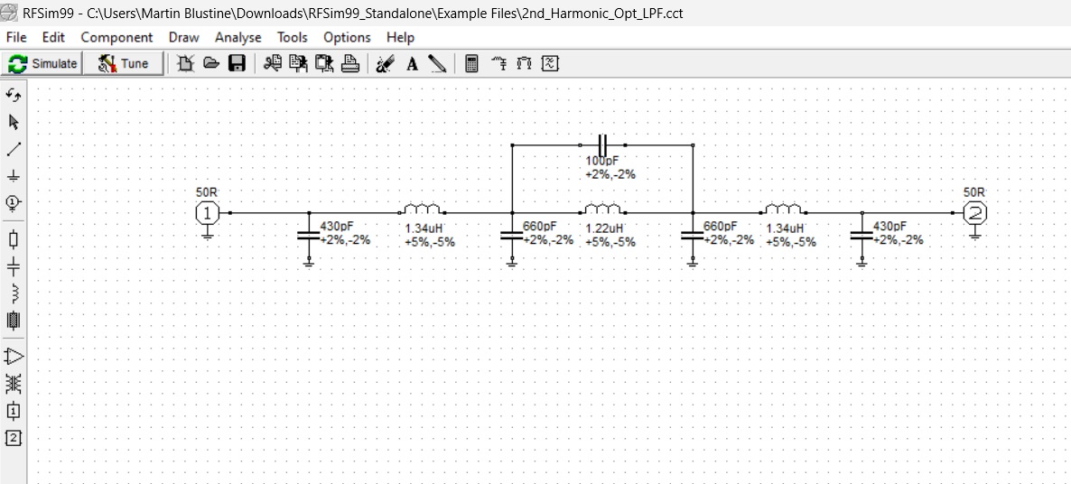
The circuit model for the 2nd harmonic optimized 40m lowpass filter is shown in Figure 4. No changes were made to the component values appearing in the original article. A parallel resonant LC in the center of the schematic resonates at the 2nd harmonic, 14.4 MHz. This serves as a high impedance at the 2nd harmonic.
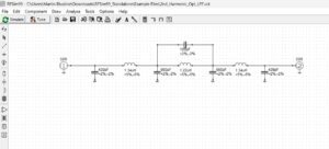
Figure 4. Circuit Model for 40m Lowpass Filter Simulation. No changes were made to the original component values in this simulation. Please note the LC circuit at the center of the schematic. It is designed to resonate at the second harmonic, 14.4 MHz. This serves as a high impedance at the 2nd harmonic.
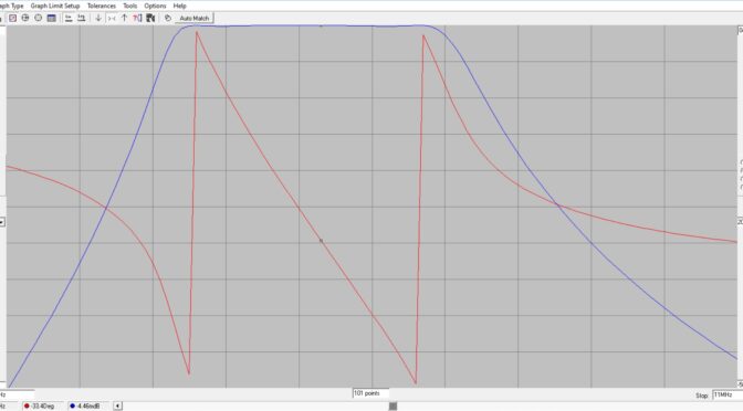
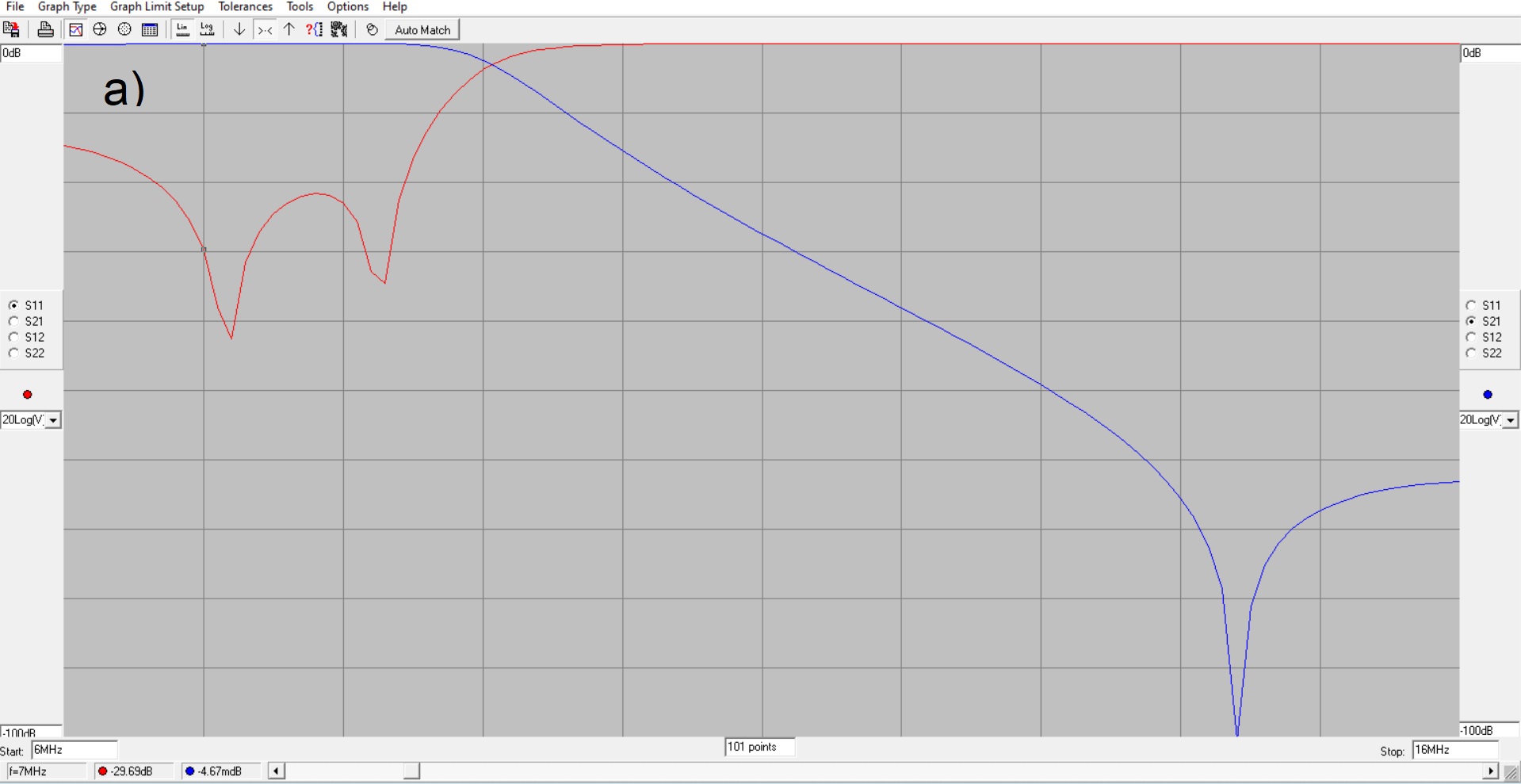
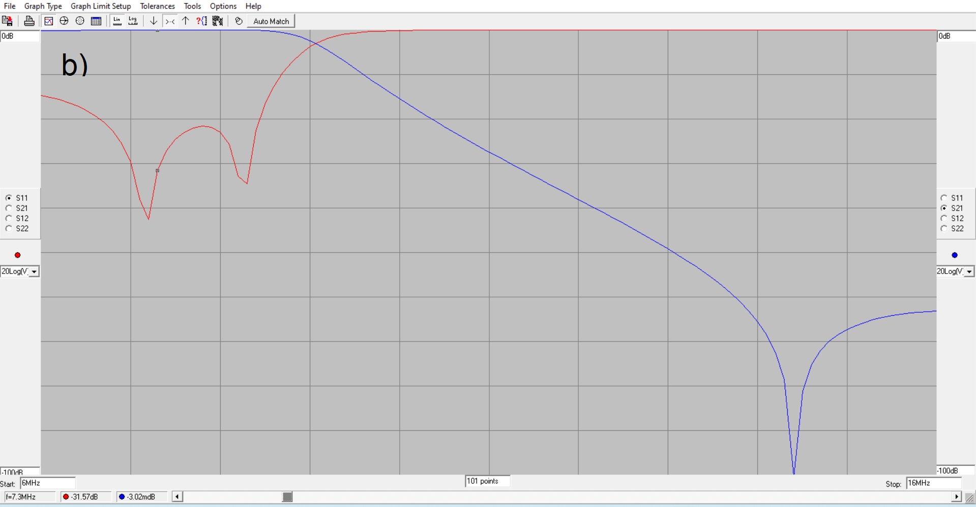
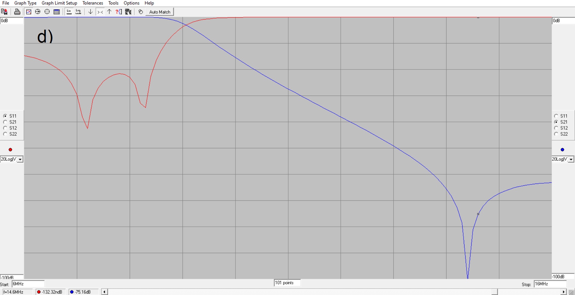
The results of the simulation are provided in Figure 5 for filter attenuation and return loss in the passband and 2nd harmonic stopband. A return loss of 29 dB corresponds to a VSWR better than 1.1:1. The attenuation at the 2nd harmonic of the 40m band will far exceed the FCC requirement of 43 dB below the mean power of carrier emission.

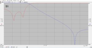
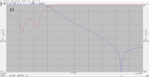
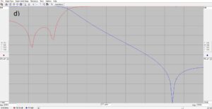
Figure 5. Simulation for the 2nd Harmonic Optimized 40m Lowpass Filter. The cursor shows where the measurement values to the left and right hand side of the plots originate; at a) the values at 7.0 MHz, at b) the values at 7.3 MHz, at c) the values at the 2nd harmonic of 7.0 MHz, at d) the values at the 2nd harmonic of 7.3 MHz. S11 is the return loss trace while S21 is the transmission trace. A return loss of 29 dB corresponds to a VSWR better than 1.1:1. The attenuation at the 2nd harmonic of the 40m band will far exceed the FCC requirement of 43 dB below the mean power of carrier emission.
Simulation of a Butterworth Bandpass Filter
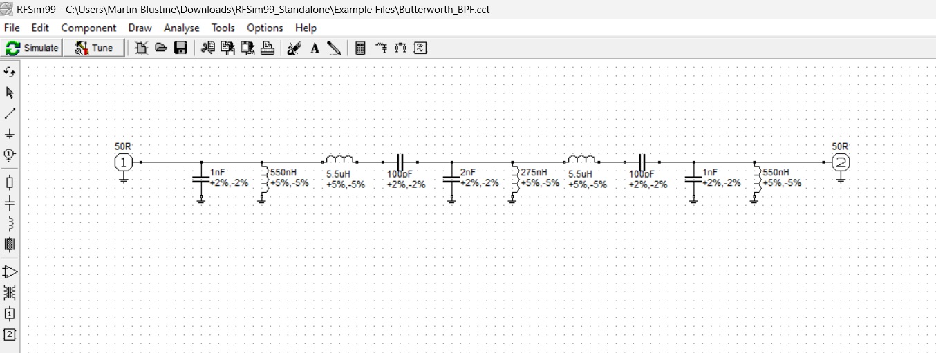
A simulation was run on a design provided by Lew Gordon, K4VX (SK), in his QST article[8]. A Butterworth bandpass filter, a.k.a. maximally flat filter, exhibits no ripples in its passband. Consequently, the stopband attenuation is more gradual than it is for other filter prototypes. (The Bessel filter also exhibits no passband ripple.) Figure 6 shows model employed for the 5-pole Butterworth bandpass filter simulation for the 40m band.
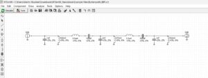 Figure 6. Simulation Model for a 40m 5-Pole Butterworth Bandpass Filter. A 5-pole filter is, essentially, two 3-pole filters back-to-back. The 2nf capacitor at the center of the filter is equivalent to 2 x 1nf capacitors in parallel. The 275nH inductor at the center of the filter is equivalent to 2 x 550nH inductors in parallel.
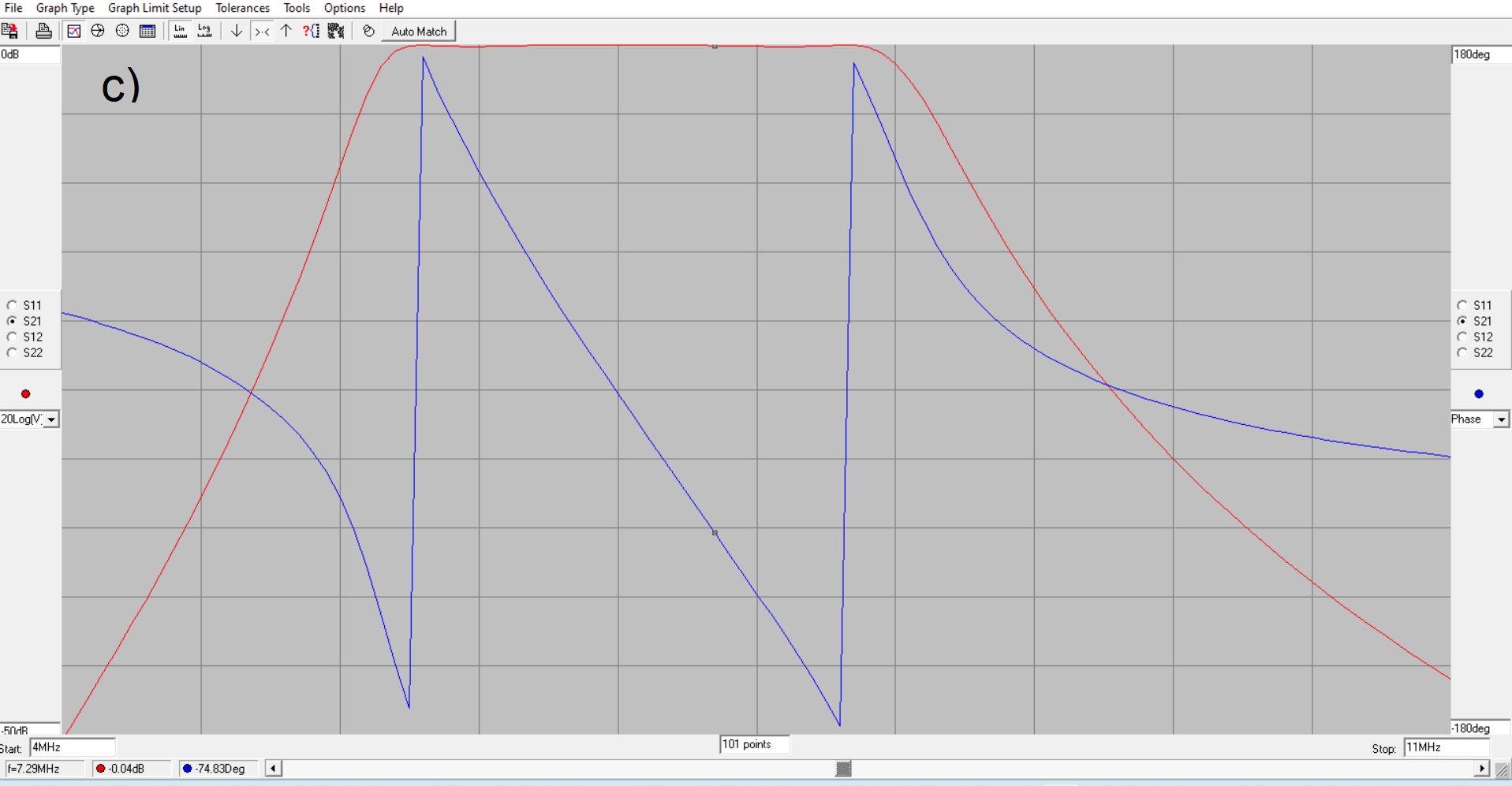
The 5-pole Butterworth bandpass filter was modeled in RFSim99, which resulted in the plots shown in Figure 7. Problems associated with the linear phase response of this filter are often avoided by deliberately making this filter very wide in which case only the center of the filter is used.
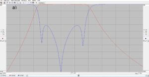
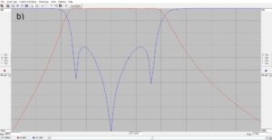
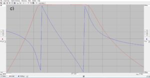
Figure 7. A 40m 5-pole Butterworth bandpass filter. At a) the filter return loss and transmission characteristics at 7.0 MHZ, at b) the filter return loss and transmission characteristics at 7.3 MHz, at c) the transmission characteristics and phase response of the filter. The filter is usually used at band center and within the linear phase region of its response. S11 is the return loss trace while S21 is the transmission trace. A return loss of 20 dB is 1.22:1.
Conclusions
The RFSim99 app is easy to use and configure. It runs reasonably well in Windows 11 when the compatibility mode for Windows XP is employed. It should run in earlier operating systems, too. There is no installer package for RFSim99 other than the one for Windows XP but AD5GG has extracted all of the files required to permit this program to run as a standalone app. Some common passive networks were analyzed that explore the capabilities of this software. Although the optimization utilities were not used for these analyses, they should be useful.
References
[1] Stewart Hyde, author, 1999.
[2] AD5GG, https://www.ad5gg.com/2017/04/06/free-rf-simulation-software/
[3] Ibid.
[4] M. Blustine, Highly Efficient L-Matching Networks for End-Fed Half-Wave Antennas, N1FD, June 11, 2022. https://www.n1fd.org/author/k1fql/page/5/
[5] Ed Wetherhold, Second-Harmonic-Optimized Low-Pass Filters, QST, February 1999, pp. 44-46. https://www.arrl.org/files/file/Technology/tis/info/pdf/9902044.pdf
[6] https://qrp-labs.com/
[7] https://easyeda.com/
[8] Lew Gordon, Band-Pass Filters for HF Transceivers, QST, September 1988, pp. 17-19, 23. https://www.arrl.org/files/file/Technology/tis/info/pdf/8809017.pdf

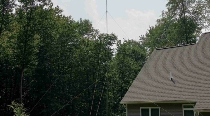
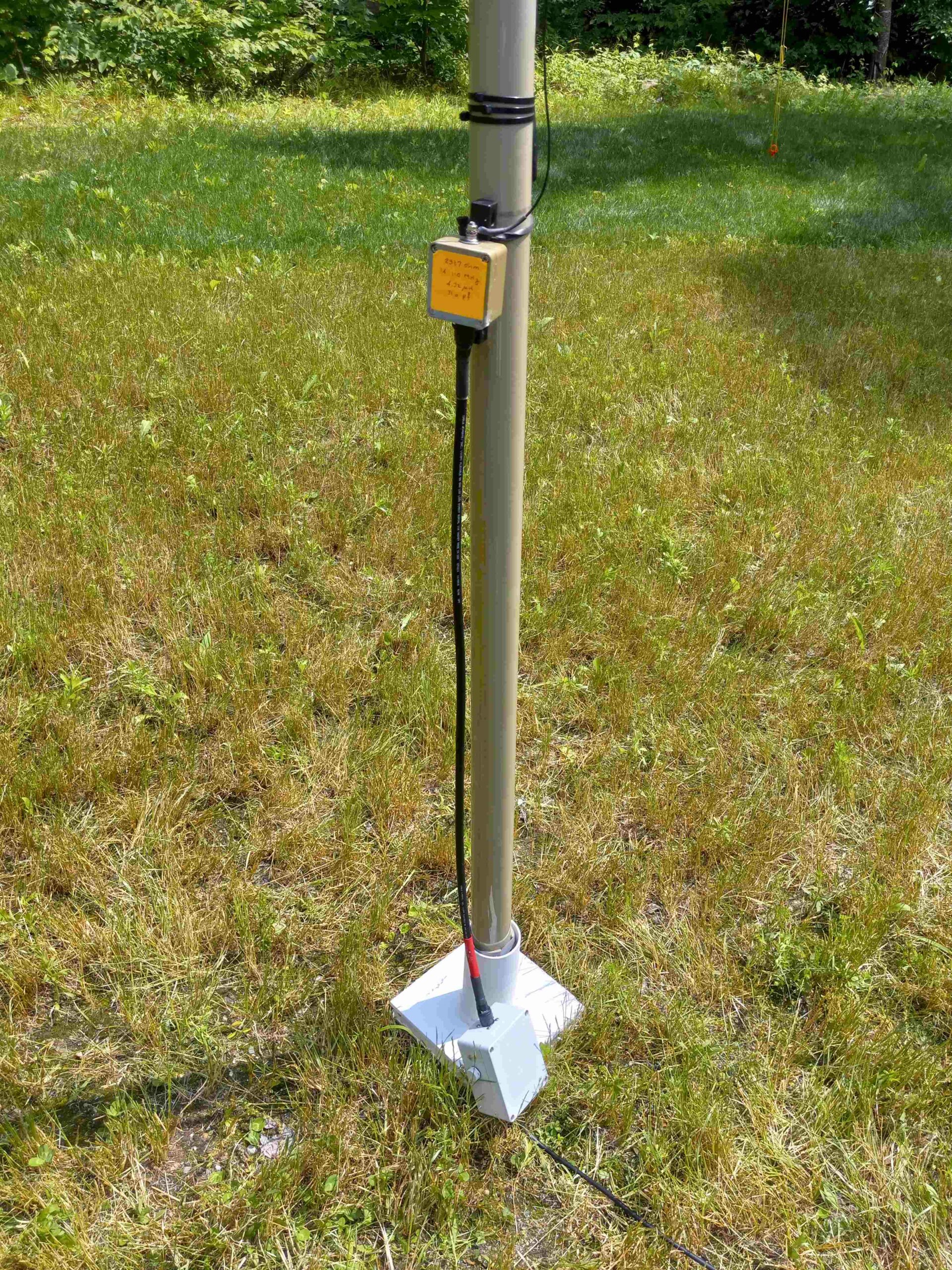 Figure 2. Matching Network, Coaxial Shield Counterpoise and Line Choke. The matching network was designed for 14.1 MHz. Since the matching network has a wide bandwidth, the antenna wire was cut slightly longer to resonate at the very bottom of the CW band. Please click on the photo to enlarge it.
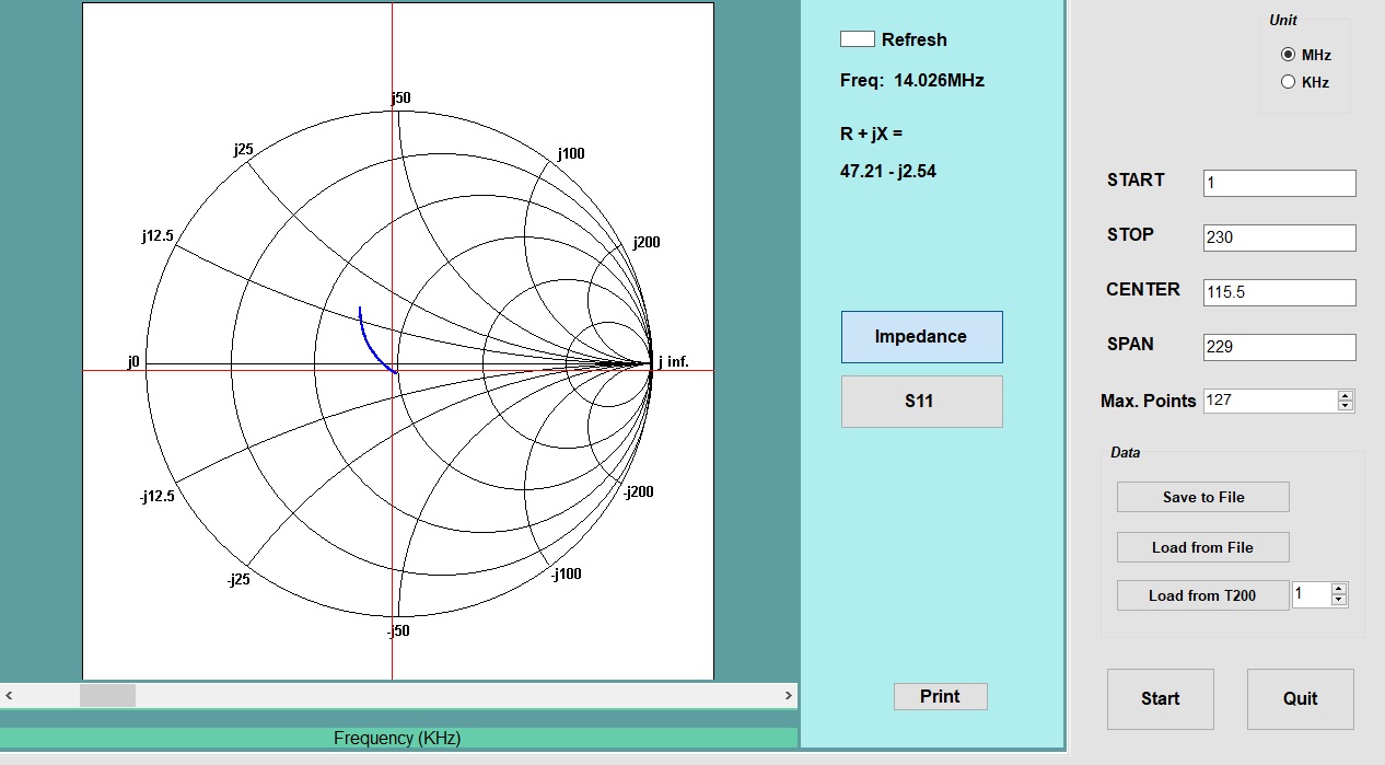 Figure 3. Smith Chart for 20m L-Matched EFHW Antenna. A match better than 2:1 match is achieved over the entire 20m band. The antenna wire was cut longer to provide the best match at 14.025 MHz. Please click on the photo to enlarge it.
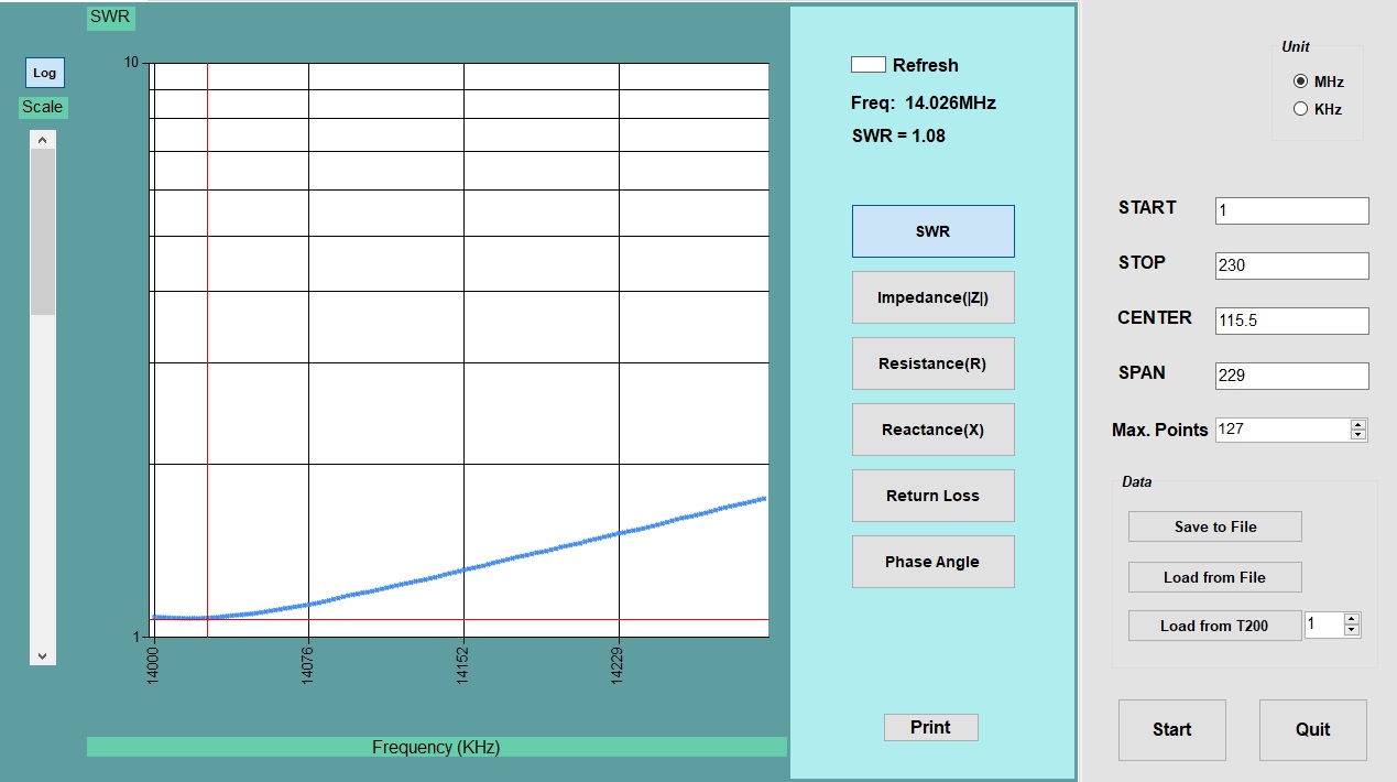 Figure 4. 20m VSWR Plot. The L-matching network exhibits wide bandwidth and good efficiency. The antenna wire is cut to resonate at the very bottom of the CW band where I like to operate. The match is very good but not perfect. This was due to the residual VSWR in the lightning arrestor located in the service entrance panel. Please click on the photo to enlarge it.