I enjoy homebrewing, and when it was time to calibrate the Stockton Bridge for measuring forward and reflected power in my QRP rig, I realized that I didn’t have a set of mismatches that could be used for that purpose. A set of mismatches is also useful for checking an SWR meter, or a nanoVNA. There are off-the-shelf mismatches that you can buy to test your nano, but they do not provide the power handling capability that this design does.

If you would like to get started with PCB design, this might be a perfect project to begin with. I am not endorsing any particular PCB design tool that you might find online, but I have found that EasyEDA is easy to learn.

The mismatches that I describe here can be used for QRP. All resistors in the design are 51-ohms and 2 Watts. Since we are not using 50-ohm resistors, this will result in a small error. Also, the layout is distributed (spread out), and this will result in a bit of extra capacitive reactance for the larger mismatches. SMA connectors were chosen because all of the RF interconnections within my QRP rig consist of RG316 terminated with SMA connectors.

Figure 1 is the schematic of what was built. It seemed pretty easy to construct the mismatches from a single value of resistor, but there is nothing to stop you from building mismatches from one or two parallel values of different resistors. What I have here seemed like a good idea because it made calculations simpler, and it resulted in power-handling capability large enough for any QRP project that I envisioned. Values of 3.0:1, 2.5:1, 2.0:1, 1.5:1 and 1.0:1 were chosen as data points for the Stockton Bridge that I was calibrating. For continuous operation at 5W, a cooling fan is recommended, particularly for the 1.0:1 load bank as it has the fewest number of resistors.

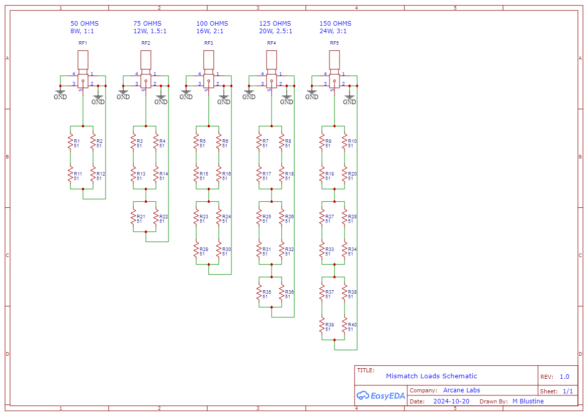Figure 1. A Simple Set of Mismatches. Use of a single resistor value, 51-ohms and 2 Watts throughout, makes construction easy and economical. Use of series and parallel combinations result in higher power dissipations. Please click on the figure to enlarge it.

Figure 2 shows the virtual 3-D layout as provided by the EasyEDA PCB layout tool. The tool shows you what you are going to get once the PCB is assembled. The EasyEDA library is extensive, and it provides additional capability to import manufacturer’s symbols and footprints not already in the library. Although this set of mismatches was built as a PCB, there is nothing to stop you from building the same design on a piece of copper-clad perforated board.

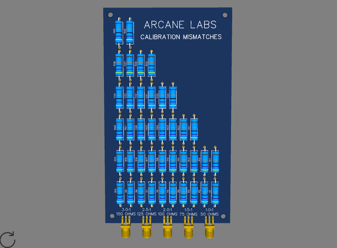Figure 2. Calibration Mismatches 3-D View. EasyEDA provides a 3-D viewer so that you can see what the final product will look like before the PCB is fabricated and before the PCB is populated. The mismatch values are shown near the SMA connectors. Please click on the figure to enlarge it.

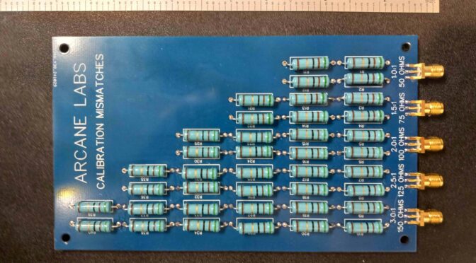
Figure 3 shows the shows the final product after PCB fabrication and population. It closely matches what is shown in Figure 2.

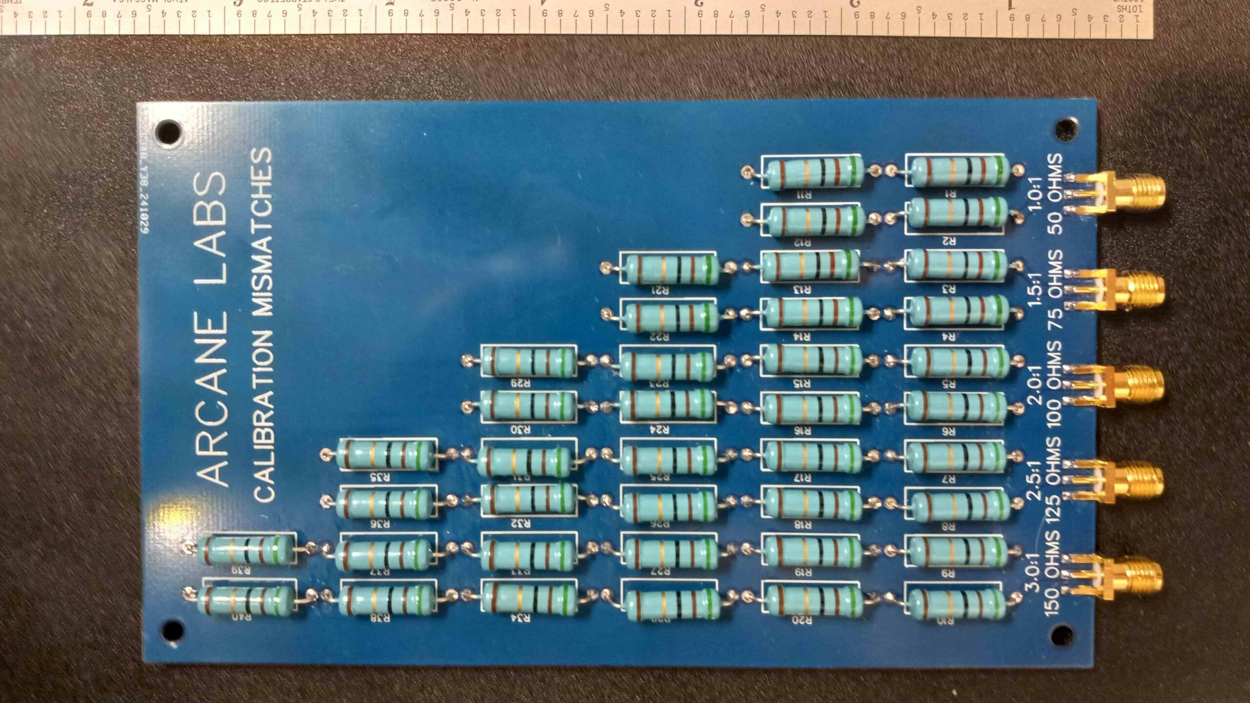
Figure 3. As-Built Calibration Mismatches. The actual PCB closely resembles the 3-D model shown in Figure 2. The overall dimensions of the completed board are 6.50” x 3.60” including the connectors. Please click on the figure to enlarge it.

S11 values for the mismatches were measured from 1.8 to 29.7 MHz and stored on an old MFJ-226 Graphical Analyzer. The values were converted to rectangular form in Excel spreadsheets to facilitate calculations. Smith Charts were also plotted. In order to make this article more concise, the Smith Charts are provided in the Appendix that follows.

If you would like the S11 data in the form of Excel, please contact me. The spreadsheets contain all of the formulas required to convert S11 magnitude and angle to other useful forms including S11 rectangular, impedance rectangular, impedance polar, VSWR and return loss.

If you would like the Gerber file for PCB fabrication, you may also contact me.  I will not be providing any bare boards, although you may wish to pool a PCB order to distribute the shipping costs among a few hams. For the JLCPCB supplier, the minimum number of boards is 5.

Appendix A. Smith Charts

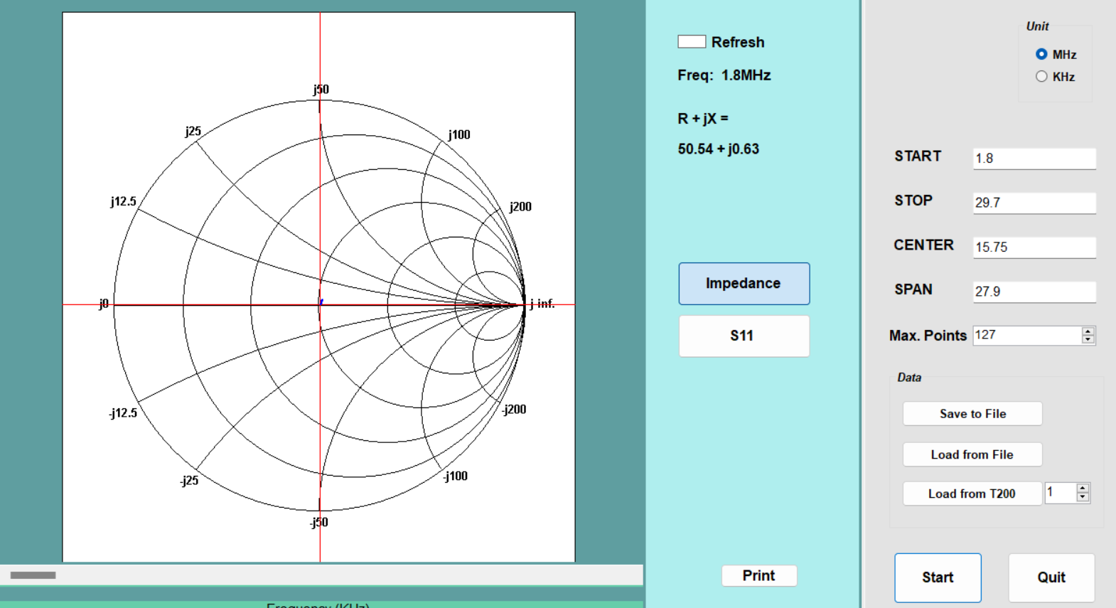
Figure A-1. Smith Chart 1.0:1 Mismatch.

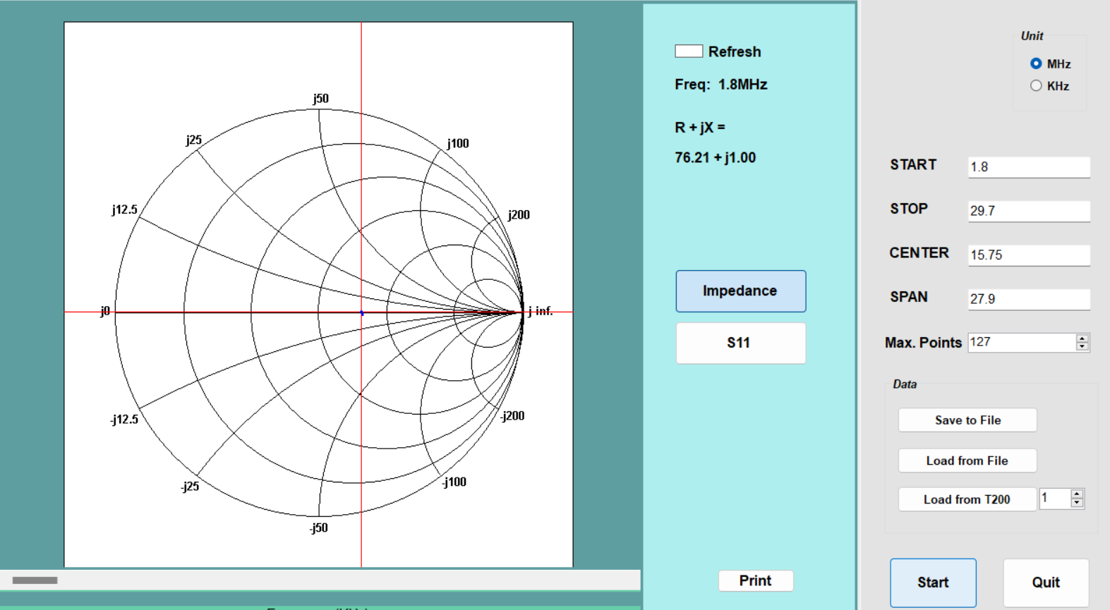
Figure A-2. Smith Chart 1.5:1 Mismatch.

Figure A-3. Smith Chart 2.0:1 Mismatch.

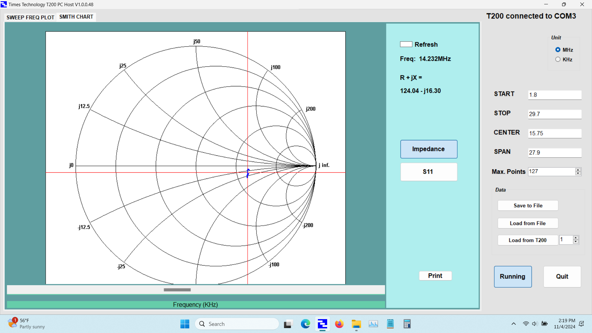
Figure A-4. Smith Chart 2.5:1 Mismatch.

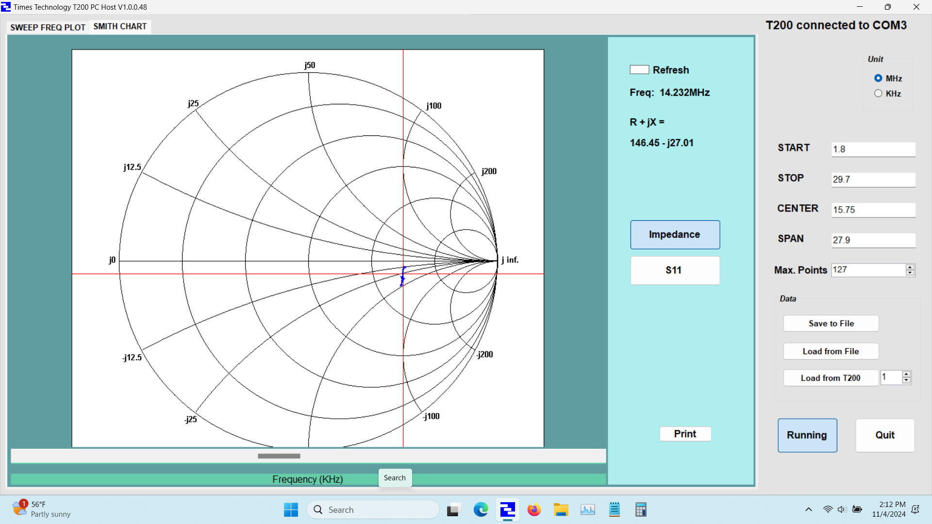
Figure A-5. Smith Chart 3.0:1 Mismatch.